All Images
Before we Start
Figure 1
Getting to know the dataTaking a look at the data
Figure 1
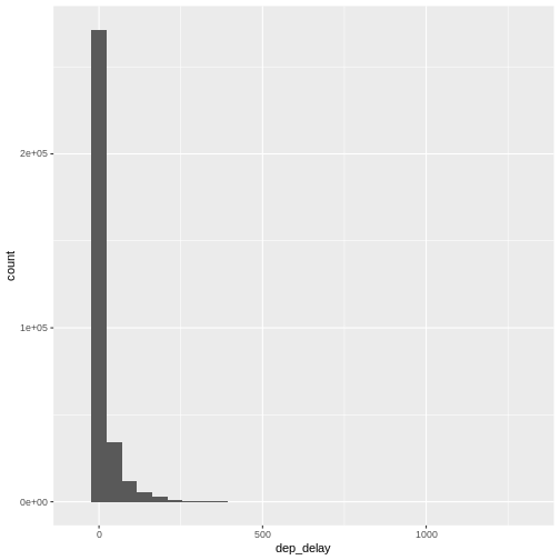 A histogram divides the numeric values of the departure delay into
“buckets” with a fixed width. It then counts the number of observations
in each bucket, and plot a column matching that count.
A histogram divides the numeric values of the departure delay into
“buckets” with a fixed width. It then counts the number of observations
in each bucket, and plot a column matching that count.
Figure 2
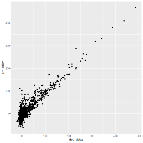
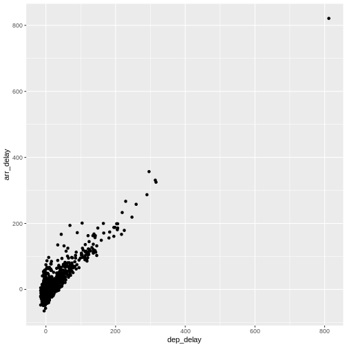 We pipe the data to
 sample_frac in order to look at 0.5% of
the data. The result of that is piped to the ggplot
function, where we specify that the data should be mapped
to the plot, by placing the values of the delay of departure on the
X-axis, and the delay of arrival on the Y-axis.
Figure 3
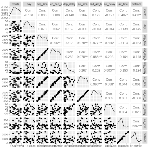
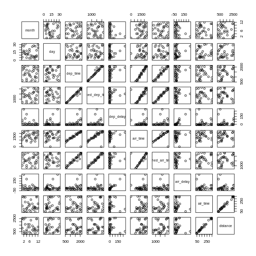 This gives us a good first indication of how the different variables
varies together. The name of this type of plot is
This gives us a good first indication of how the different variables
varies together. The name of this type of plot is
correllogram because it shows all the correlations between
the selected variables.
Figure 4
Exploring with summary statistics
Joining data
Figure 1
 .
.
Figure 2
Boxplots and linear regressions
Figure 1
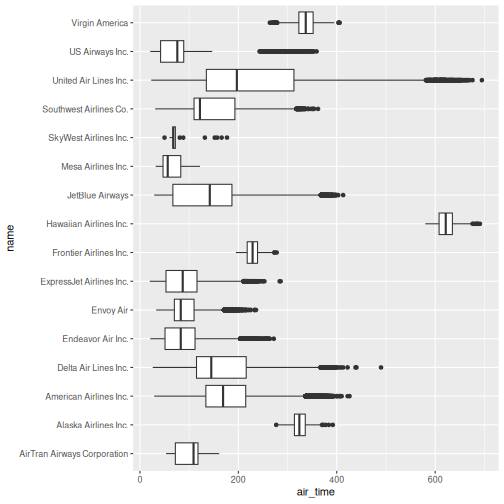
Figure 2
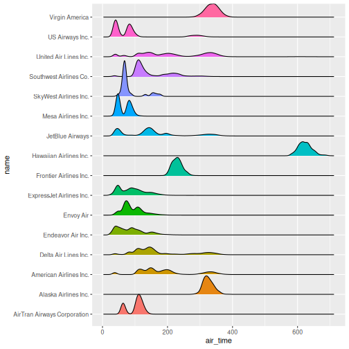 The number of flights United Air Lines have to Hawaii is too low to
actually see here. But we do get a more nuanced view of the distribution
of airtime for the individual airlines than we do using boxplots.
The number of flights United Air Lines have to Hawaii is too low to
actually see here. But we do get a more nuanced view of the distribution
of airtime for the individual airlines than we do using boxplots.
Figure 3
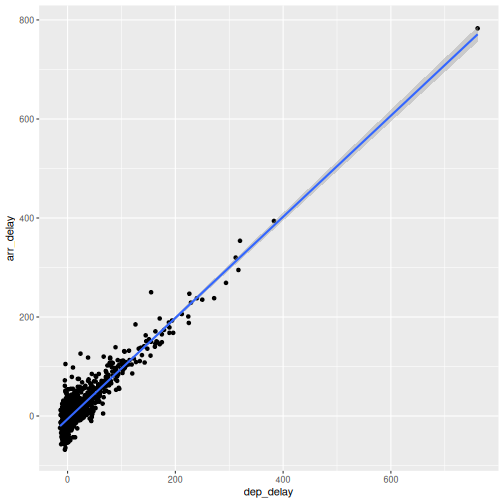
 This looks more or less linear. We can place a linear regression line in
the plot using the function
This looks more or less linear. We can place a linear regression line in
the plot using the function geom_smooth(method = "lm"),
where we specify that the function should fit a linear line to the
data.
Figure 4
 So, what is the actual linear model of this data?