The normal distribution
Last updated on 2026-06-08 | Edit this page
Estimated time: 12 minutes
Overview
Questions
- What even is a normal distribution?
Objectives
- Explain how to use markdown with the new lesson template
- Demonstrate how to include pieces of code, figures, and nested challenge blocks
Inline instructor notes can help inform instructors of timing challenges associated with the lessons. They appear in the “Instructor View”
What is the normal distribution
A probability distribution is a mathematical function, that describes the likelihood of different outcomes in a random experiment. It gives us probabilities for all possible outcomes, and is normalised so that the sum of all the probabilities is 1.
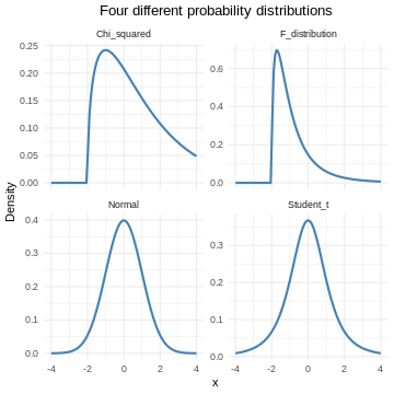
Probability distributions can be discrete, or they can be continuous. The normal distribution is just one of several different continuous probability distributions.
The normal distribution is especially important, for a number of reasons:
If we take a lot of samples from a population and calculate the averages of a given variable in those samples, the averages, or means will be normally distributed. This is know as the Central Limit Theorem.
Many natural (and human made) processes follow a normal distribution.
The normal distribution have useful mathematical properties. It might not appear to be simple working with the normal distribution. But the alternative is worse.
Many statistical methods and tests are based on assumptions of normality.
How does it look - mathematically?
The normal distribution follows this formula:
\[ f(x) = \frac{1}{\sqrt{2\pi\sigma^2}} e^{-\frac{(x-\mu)^2}{2\sigma^2}} \]
If a variable in our population is normally distributed, have a mean \(\mu\) and a standard deviation \(\sigma\), we can find the probability of observing the value \(x\) of the varibel by plugging in the values, and calculate \(f(x)\).
Note that we are here working with the population mean and standard deviation. Those are the “true” mean and standard deviation for the entire universe. That is signified by using the greek letters \(\mu\) and \(\sigma\). In practise we do not know what those true values are.
What does it mean that our data is normally distributed
We have an entire section on that - but in short: The probabilities we get from the formula above should match the frequencies we observe in our data.
How does it look- graphically?
It is useful to be able to compare the distributions of different variables. That can be difficult if one have a mean of 1000, and the other have a mean of 2. Therefore we often work with standardized normal distributions, where we transform the data to have a mean of 0 and a standard deviation of 1. So let us look at the standardized normal distribution.
If we plot it, it looks like this:
 The area under the curve is 1,
equivalent to 100%.
The area under the curve is 1,
equivalent to 100%.
The normal distribution have a lot of nice mathematical properties, some of which are indicated on the graph.
So - what is the probability?
The normal distribution curve tell what the probability density for a given observation is. But in general we are interested in the probability that something is larger, or smaller, than something. Or between certain values.
Rather that plotting the probability density, we can plot the cumulative density.
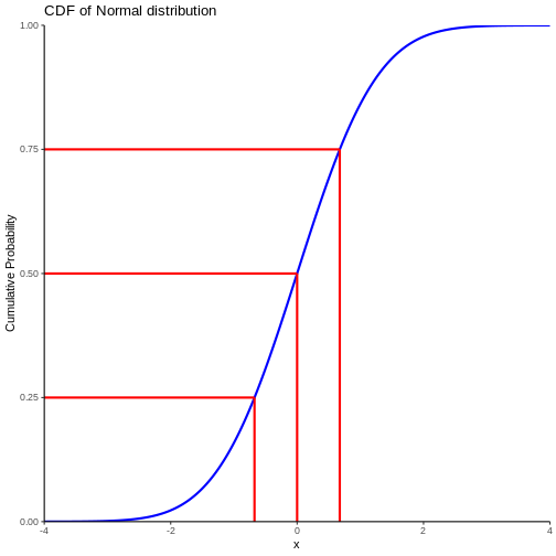
Note that we also find the cumulitive probability in the original plot of the normal distribution - now it is a bit more direct.
This allow us to see that the probability of observing a value that is 2 standard deviations smaller than the mean is rather small.
We can also, more indirectly, note that the probability of observing a value that is 2 standard deviations larger than the mean is rather small. Note that the probability of an observation that is smaller than 2 standard deviations larger than the mean is 97.7% (hard to read on the graph, but we will get to that). Since the total probability is 100%, the probability of an observation being larger than 2 standard deviations is 100 - 97.7 = 2.3%
Do not read the graph - do the calculation
Instead of trying to measure the values on the graph, we can do the calculations directly.
R provides us with a set of functions:
- pnorm returns the probability of having a smaller value than x
- qnorm the value x corresponding to a given probability
- dnorm returns the probability density of the normal distribution at a given x.
We have an additional rnorm that returns a random value, drawn from a normal distribution.
Try it your self!
Assuming that our observations are normally distributed with a mean of 0 and a standard deviation of 1.
What is the probability of an observation x < 2?
R
pnorm(2)
OUTPUT
[1] 0.9772499About 98% of the observations are smaller than 2
Challenge
Making the same assumptions, what is the value of the observation, for which 42% of the observations is smaller?
R
qnorm(0.42)
OUTPUT
[1] -0.201893542% of the observations are smaller than -0.2
What about other means and standard deviations?
Being able to find out what the probablity of some observation being smaller when the mean is 0 and the standard deviation is 1, is nice. But this is not a common problem.
Rather we might know that adult men in a given country have an average height of 183 cm, and that the standard deviation of their height is 9.7 cm.
What is the probability to encounter a man that is taller than 2 meters?
The R-functions handle this easily, we “simply” specify the mean and standard deviation in the function:
R
1 - pnorm(200, mean = 183, sd = 9.7)
OUTPUT
[1] 0.03983729The function calculate the probability of a man being shorter than 200 cm, if the distribution is normal and the mean and standard devation is 183 and 9.7 respectively. The probability of the man having a height is 1 (equivalent to 100%). So if the probability of the man being shorter than 200 cm is 96%, the probability of him being taller than 200 cm is 4%
We have a lot of men with an average height of 183. They all have an individual heigth. If we subtract 183 from their height, and use that as a measurement of their height, that will have a mean of 0.
We are not going into the details, but if we divide all the heights with the original standard deviation, and do all the math, we will discover that the standard deviation of the new heights will be 1.
Therefore, if we subtract 183 from all the individual heights, and divide them by 9.7, the resulting measurements of the heights have a mean of 0 and a standard deviation of 1. Bringing all that together, we get:
R
1 - pnorm((200-183)/9.7)
OUTPUT
[1] 0.03983729How many men are in an interval?
How many men have a height between 170 and 190 cm?
Assume mean = 183 cm and sd = 9.7
What proportion of men are shorter than 190 cm? And what proportion of men are shorter than 170 cm?
R
pnorm(190, mean =183, sd = 9.7 ) - pnorm(170, mean = 183, sd = 9.7)
OUTPUT
[1] 0.6746558CLT
But my data is not normally distributed?
No, it is not. Actually most data is not normally distributed. Often it cannot be normally distributed. Serum molybdenum, an essential trace metal in human physiology has a mean of 1.55 and a standard deviation of 0.74 in normal healthy adult humans.
How many danes have negative serum molybdenum?
Assuming an adult population of 5000000 danes, a mean of 1.55 and a standard deviation of 0.74, how many danes have a negative concentration of Molybdenum (Mo) in their blood?
We begin by calculating the probability of observing a Mo concentration lower than 0:
R
pnorm(0, mean = 1.55, sd = 0.74)
OUTPUT
[1] 0.01810352We then multiply by the number of people:
R
5000000*0.01810352
OUTPUT
[1] 90517.6About 90000 adult danes have not only none, but actually negative amounts of Molybdenum in their blood. Which is impossible.
So - your data is not normally distributed. But the properties of your samples are!
We are not actually measuring the average height of all men in the world ever. We are taking a sample, and calculating the mean. And standard deviation. And proportion.
And those, the mean etc, are normally distributed, even if the underlying distribution of the population is not.
The Central Limit Theorem allow us to assume that, if we take enough random samples, the mean and standard deviation of these samples, will be normally distributed.
This is what we use when doing statistical tests. We posit a null-hypothesis that the “true” mean of some value should be something. We take a sample, and calculate the mean. And using the normal distribution, we can look at the CDF-plot above, and determine the probability of seeing the value we get.
In practice we are usually not using the normal distribution, buth rather the t-distribution, to correct for the fact that we do not actually know the true mean and varians/standard deviation of the population. It gives us a more conservative estimate taht is more likely to be “true”.
What is normal?
The normal distribution is normal, because Karl Pearson and Francis Galton in the 19th century took a lot of samples of different phenomenons in the population data. Height, weight, intelligence etc. Calculating the mean (and other descriptive statistical parameters) they noted that these means followed a specific distribution. This was not the case for every phenomenon. But for a lot.
Looking at the distributions describing a lot of phenomenons, the most common was one specific distribution.
In descriptive statistics, the normal observation is simply the most frequent. In this set of numbers:
OUTPUT
[1] 1 2 3 4 5 55 is the normal observation - because it is the most frequent, even if it only represents 20% of the observations. In a statistical sense normal is not normative. The normal colour eye among humans is brown. Not because there is anything wrong with other colours, but simply because brown is the most frequent.
The most frequent, ie normal, distribution found, was named the normal distribution.
- Use
.mdfiles for episodes when you want static content - Use
.Rmdfiles for episodes when you need to generate output - Run
sandpaper::check_lesson()to identify any issues with your lesson - Run
sandpaper::build_lesson()to preview your lesson locally