Introduction to R: All in One View

Last updated on 2024-04-30 | Edit this page

Overview

Questions

How to find your way around RStudio?
How to interact with R?
How to manage your environment?
How to install packages?

Objectives

Install latest version of R.
Install latest version of RStudio.
Navigate the RStudio GUI.
Install additional packages using the packages tab.
Install additional packages using R code.

What is R? What is RStudio?

The term “R” is used to refer to both the programming language and the software that interprets the scripts written in R.

RStudio is currently a very popular way to not only write your R scripts but also to interact with the R software. RStudio is the most popular IDE (Integrated Development Environmemt) for R. An IDE is a piece of software that provides tools to make programming easier.

To make it easier to interact with R, we will use RStudio. To function correctly, RStudio needs R and therefore both need to be installed on your computer.

Why learn R?

There are numerous reasons to learn and use R. In the following we will point out a few of them.

R does not involve lots of pointing and clicking

The learning curve might be steeper than with other software, but with R, the results of your analysis do not rely on remembering a succession of pointing and clicking, but instead on a series of written commands, and that’s a good thing! So, if you want to redo your analysis because you collected more data, you don’t have to remember which button you clicked in which order to obtain your results; you just have to run your script again.

Working with scripts makes the steps you used in your analysis clear, and the code you write can be inspected by someone else who can give you feedback and spot mistakes.

Working with scripts forces you to have a deeper understanding of what you are doing, and facilitates your learning and comprehension of the methods you use.

R code is great for reproducibility

Reproducibility is when someone else (including your future self) can obtain the same results from the same dataset when using the same analysis.

R integrates with other tools to generate manuscripts from your code. If you collect more data, or fix a mistake in your dataset, the figures and the statistical tests in your manuscript are updated automatically.

An increasing number of journals and funding agencies expect analyses to be reproducible, so knowing R will give you an edge with these requirements.

R is interdisciplinary and extensible

With 18,000+ packages that can be installed to extend its capabilities, R provides a framework that allows you to combine statistical approaches from many scientific disciplines to best suit the analytical framework you need to analyze your data. For instance, R has packages for image analysis, GIS, time series, population genetics, and a lot more.

R works on data of all shapes and sizes

The skills you learn with R scale easily with the size of your dataset. Whether your dataset has hundreds or millions of lines, it won’t make much difference to you.

R is designed for data analysis. It comes with special data structures and data types that make handling of missing data and statistical factors convenient.

R can connect to spreadsheets, databases, and many other data formats, on your computer or on the web.

R produces high-quality graphics

The plotting functionalities in R are endless, and allow you to adjust any aspect of your graph to convey most effectively the message from your data.

R has a large and welcoming community

Thousands of people use R daily. Many of them are willing to help you through mailing lists and websites such as Stack Overflow, or on the Posit Community. Questions which are backed up with short, reproducible code snippets are more likely to attract knowledgeable responses.

Not only is R free, but it is also open-source and cross-platform

Anyone can inspect the source code to see how R works. Because of this transparency, there is less chance for mistakes, and if you (or someone else) find some, you can report and fix bugs.

Because R is open source and is supported by a large community of developers and users, there is a very large selection of third-party add-on packages which are freely available to extend R’s native capabilities.

automatic car gear shift representing the ease of RStudio

RStudio extends what R can do, and makes it easier to write R code and interact with R. Left photo credit; Right photo credit.

A tour of RStudio

Let’s start by learning about RStudio, which is an Integrated Development Environment (IDE) for working with R.

The RStudio IDE open-source product is free under the Affero General Public License (AGPL) v3. The RStudio IDE is also available with a commercial license and priority email support from Posit Software, Inc.

We will use the RStudio IDE to write code, navigate the files on our computer, inspect the variables we create, and visualize the plots we generate. RStudio can also be used for other things (e.g., version control, developing packages, writing Shiny apps) that we will not cover during the workshop.

One of the advantages of using RStudio is that all the information you need to write code is available in a single window. Additionally, RStudio provides many shortcuts, autocompletion, and highlighting for the major file types you use while developing in R. RStudio makes typing easier and less error-prone.

The RStudio Interface

Let’s take a quick tour of RStudio.

RStudio is divided into four “panes”. The placement of these panes and their content can be customized (see menu, Tools -> Global Options -> Pane Layout).

The Default Layout is: - Top Left - Source: your scripts and documents - Bottom Left - Console: what R would look and be like without RStudio - Top Right - Enviornment/History: look here to see what you have done - Bottom Right - Files and more: see the contents of the project/working directory here, like your Script.R file

Getting set up

It is good practice to keep a set of related data, analyses, and text self-contained in a single folder called the working directory. All of the scripts within this folder can then use relative paths to files. Relative paths indicate where inside the project a file is located (as opposed to absolute paths, which point to where a file is on a specific computer). Working this way makes it a lot easier to move your project around on your computer and share it with others without having to directly modify file paths in the individual scripts.

RStudio provides a helpful set of tools to do this through its “Projects” interface, which not only creates a working directory for you but also remembers its location (allowing you to quickly navigate to it). The interface also (optionally) preserves custom settings and open files to make it easier to resume work after a break.

An easy way to work like this is to create projects in RStudio.

Create a new project and a new script file

Under the File menu, click on New project, choose New directory, then New project
Enter a name for this new folder (or “directory”) and choose a convenient location for it. This will be your working directory for working on this project (e.g., ~/data-carpentry)
Click on Create project
Create a new file where we will type our scripts. Go to File > New File > R script. Click the save icon on your toolbar and save your script as “script.R”.

The simplest way to open an RStudio project once it has been created is to navigate through your filesystem to where the project was saved and double click on the .Rproj (blue cube) file. This will open RStudio and start your R session in the same directory as the .Rproj file. All your data, plots and scripts will now be relative to the project directory. RStudio projects have the added benefit of allowing you to open multiple projects at the same time each open to its own project directory. This allows you to keep multiple projects open without them interfering with each other.

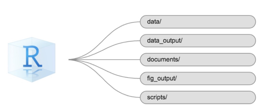
Organizing your working directory

Using a consistent folder structure across your projects will help keep things organized and make it easy to find/file things in the future. This can be especially helpful when you have multiple projects. In general, you might create directories (folders) for scripts, data, and documents. Here are some examples of suggested directories:

data/ Use this folder to store your raw data and intermediate datasets. For the sake of transparency and provenance, you should always keep a copy of your raw data accessible and do as much of your data cleanup and preprocessing programmatically (i.e., with scripts, rather than manually) as possible.
data_output/ When you need to modify your raw data, it might be useful to store the modified versions of the datasets in a different folder.
documents/ Used for outlines, drafts, and other text.
fig_output/ This folder can store the graphics that are generated by your scripts.
scripts/ A place to keep your R scripts for different analyses or plotting.

You may want additional directories or subdirectories depending on your project needs, but these should form the backbone of your working directory.

A picture showing the layout of a good working directory as described above

The working directory

The working directory is an important concept to understand. It is the place where R will look for and save files. When you write code for your project, your scripts should refer to files in relation to the root of your working directory and only to files within this structure.

Using RStudio projects makes this easy and ensures that your working directory is set up properly. If you need to check it, you can use getwd(). If for some reason your working directory is not the same as the location of your RStudio project, it is likely that you opened an R script or RMarkdown file not your .Rproj file. You should close out of RStudio and open the .Rproj file by double clicking on the blue cube!

Downloading the data and getting set up

For this lesson we will use the following folders in our working directory: data/, data_output/ and fig_output/. Let’s write them all in lowercase to be consistent. We can create them using the RStudio interface by clicking on the “New Folder” button in the file pane (bottom right), or directly from R by typing at console:

R

dir.create("data")
dir.create("data_output")
dir.create("fig_output")

Begin by downloading the dataset called “movieSerie.csv”. Place this downloaded file in the data/ you just created. You can do this directly from R by copying and pasting this in your terminal (your instructor can place this chunk of code in the Etherpad):

R

download.file("https://raw.githubusercontent.com/KUBDatalab/R-intro/main/episodes/data/movieSerie.csv", "data/movieSerie.csv", mode = "wb")

Interacting with R

The basis of programming is that we write down instructions for the computer to follow, and then we tell the computer to follow those instructions. We write, or code, instructions in R because it is a common language that both the computer and we can understand. We call the instructions commands and we tell the computer to follow the instructions by executing (also called running) those commands.

There are two main ways of interacting with R: by using the console or by using script files (plain text files that contain your code). The console pane (in RStudio, the bottom left panel) is the place where commands written in the R language can be typed and executed immediately by the computer. It is also where the results will be shown for commands that have been executed. You can type commands directly into the console and press Enter to execute those commands, but they will be forgotten when you close the session.

Because we want our code and workflow to be reproducible, it is better to type the commands we want in the script editor and save the script. This way, there is a complete record of what we did, and anyone (including our future selves!) can easily replicate the results on their computer.

RStudio allows you to execute commands directly from the script editor by using the Ctrl + Enter shortcut (on Mac, Cmd + Return will work). The command on the current line in the script (indicated by the cursor) or all of the commands in selected text will be sent to the console and executed when you press Ctrl + Enter. If there is information in the console you do not need anymore, you can clear it with Ctrl + L. You can find other keyboard shortcuts in this RStudio cheatsheet about the RStudio IDE.

At some point in your analysis, you may want to check the content of a variable or the structure of an object without necessarily keeping a record of it in your script. You can type these commands and execute them directly in the console. RStudio provides the Ctrl + 1 and Ctrl + 2 shortcuts allow you to jump between the script and the console panes.

If R is ready to accept commands, the R console shows a > prompt. If R receives a command (by typing, copy-pasting, or sent from the script editor using Ctrl + Enter), R will try to execute it and, when ready, will show the results and come back with a new > prompt to wait for new commands.

If R is still waiting for you to enter more text, the console will show a + prompt. It means that you haven’t finished entering a complete command. This is likely because you have not ‘closed’ a parenthesis or quotation, i.e. you don’t have the same number of left-parentheses as right-parentheses or the same number of opening and closing quotation marks. When this happens, and you thought you finished typing your command, click inside the console window and press Esc; this will cancel the incomplete command and return you to the > prompt. You can then proofread the command(s) you entered and correct the error.

Installing additional packages using the packages tab

In addition to the core R installation, there are in excess of 18,000 additional packages which can be used to extend the functionality of R. Many of these have been written by R users and have been made available in central repositories, like the one hosted at CRAN, for anyone to download and install into their own R environment. You should have already installed the packages ‘ggplot2’ and ’dplyr. If you have not, please do so now using these instructions.

Installing additional packages using RStudio

You can see if you have a package installed by looking in the packages tab (on the lower-right by default). You can also type the command installed.packages() into the console and examine the output.

Additional packages can be installed from the ‘packages’ tab. On the packages tab, click the ‘Install’ icon and start typing the name of the package you want in the text box. As you type, packages matching your starting characters will be displayed in a drop-down list so that you can select them.

At the bottom of the Install Packages window is a check box to ‘Install’ dependencies. This is ticked by default, which is usually what you want. Packages can (and do) make use of functionality built into other packages, so for the functionality contained in the package you are installing to work properly, there may be other packages which have to be installed with them. The ‘Install dependencies’ option makes sure that this happens.

Because the install process accesses the CRAN repository, you will need an Internet connection to install packages.

It is also possible to install packages from other repositories, as well as Github or the local file system, but we won’t be looking at these options in this lesson.

Installing additional packages using R code

If you were watching the console window when you started the install of ‘tidyverse’, you may have noticed that the line

R

install.packages("tidyverse")

was written to the console before the start of the installation messages.

You could also have installed the tidyverse packages by running this command directly at the R terminal.

Challenge

Use both the Console and the Packages tab to confirm that you have the tidyverse installed.

Show me the solution

Scroll through packages tab down to ‘tidyverse’. You can also type a few characters into the searchbox. The ‘tidyverse’ package is really a package of packages, including ‘ggplot2’ and ‘dplyr’, both of which require other packages to run correctly. All of these packages will be installed automatically. Depending on what packages have previously been installed in your R environment, the install of ‘tidyverse’ could be very quick or could take several minutes. As the install proceeds, messages relating to its progress will be written to the console. You will be able to see all of the packages which are actually being installed.

In the console. If you write tidy it should put up if it is installed. Look for tidyverse::

Key Points

Use RStudio to write and run R programs.
Use install.packages() to install packages (libraries).

Content from Introduction to R

Last updated on 2024-04-30 | Edit this page

Overview

Questions

What data types are available in R?
What is an object?
How can values be initially assigned to variables of different data types?
What arithmetic and logical operators can be used?
How can subsets be extracted from vectors?
How does R treat missing values?
How can we deal with missing values in R?

Objectives

Define the following terms as they relate to R: object, assign, call, function, arguments, options.
Assign values to objects in R.
Learn how to name objects.
Use comments to inform script.
Solve simple arithmetic operations in R.
Call functions and use arguments to change their default options.
Inspect the content of vectors and manipulate their content.
Subset and extract values from vectors.
Analyze vectors with missing data.

Creating objects in R

You can get output from R simply by typing math in the console:

R

3 + 5

OUTPUT

[1] 8

R

12 / 7

OUTPUT

[1] 1.714286

However, to do useful and interesting things, we need to assign values to objects. To create an object, we need to give it a name followed by the assignment operator <-, and the value we want to give it:

R

x <- 3

<- is the assignment operator. It assigns values on the right to objects on the left. So, after executing x <- 3, the value of x is 3. The arrow can be read as 3 goes into x.

In RStudio, typing Alt + - (push Alt at the same time as the - key) will write <- in a single keystroke in a PC, while typing Option + - (push Option at the same time as the - key) does the same in a Mac.

Historical

For historical reasons, you can also use = for assignments, but not in every context. Because of the slight differences in syntax, it is good practice to always use <- for assignments. More generally we prefer the <- syntax over = because it makes it clear what direction the assignment is operating (left assignment), and it increases the read-ability of the code.

Naming objects

Objects can be given any name such as x, current_temperature, or subject_id. You want your object names to be explicit and not too long.

They cannot start with a number (2x is not valid, but x2 is), and R is case sensitive (e.g., age is different from Age). There are some names that cannot be used because they are the names of fundamental objects in R (e.g., if, else, for, see here for a complete list). In general, even if it’s allowed, it’s best to not use them (e.g., c, T, mean, data, df, weights). If in doubt, check the help to see if the name is already in use.

It is best to avoid dots (.) within an object name as in my.dataset. There are many objects in R with dots in their names for historical reasons, but because dots have a special meaning in R (for methods) and other programming languages, it’s best to avoid them.

It is also recommended to use nouns for object names, and verbs for function names. It’s important to be consistent in the styling of your code (where you put spaces, how you name objects, etc.). Using a consistent coding style makes your code clearer to read for your future self and your collaborators.

In R, three popular style guides are Google’s, Jean Fan’s and the tidyverse’s. The tidyverse’s is very comprehensive and may seem overwhelming at first. You can install the lintr package to automatically check for issues in the styling of your code.

Objects vs. variables

What are known as objects in R are known as variables in many other programming languages. Depending on the context, object and variable can have drastically different meanings. However, in this lesson, the two words are used synonymously. For more information see: https://cran.r-project.org/doc/manuals/r-release/R-lang.html#Objects

Printing objects

When assigning a value to an object, R does not print anything. You can force R to print the value by using parentheses or by typing the object name:

R

area_hectares <- 1.0    # doesn't print anything
area_hectares         # but typing the name of the object print

OUTPUT

[1] 1

R

(area_hectares <- 1.0)  # putting parenthesis around the call also print

OUTPUT

[1] 1

Doing math on objects

Now that R has area_hectares in memory, we can do arithmetic with it. For instance, we may want to convert this area into acres (area in acres is 2.47 times the area in hectares):

R

2.47 * area_hectares

OUTPUT

[1] 2.47

We can also change an object’s value by assigning it a new one:

R

area_hectares <- 2.5
2.47 * area_hectares

OUTPUT

[1] 6.175

Assigning a value to one object does not automatically change the values of other objects. For example, let’s store the plot’s area in acres in a new object, area_acres:

R

area_acres <- 2.47 * area_hectares

and then change area_hectares to 50.

R

area_hectares <- 50

Exercise

What do you think is the current content of the object area_acres? 123.5 or 6.175?

Show me the solution

The value of area_acres is still 6.175 because you have not re-run the line area_acres <- 2.47 * area_hectares since changing the value of area_hectares.

Exercise

Create two variables r_length and r_width and assign them values. It should be noted that, because length is a built-in R function, R Studio might add “()” after you type length and if you leave the parentheses you will get unexpected results. This is why you might see other programmers abbreviate common words. Create a third variable r_area and give it a value based on the current values of r_length and r_width. Show that changing the values of either r_length and r_width does not affect the value of r_area.

Show me the solution

R

r_length <- 2.5
r_width <- 3.2
r_area <- r_length * r_width
r_area

OUTPUT

[1] 8

R

# change the values of r_length and r_width
r_length <- 7.0
r_width <- 6.5
# the value of r_area isn't changed
r_area

OUTPUT

[1] 8

Comments

All programming languages allow the programmer to include comments in their code. To do this in R we use the # character. Anything to the right of the # sign and up to the end of the line is treated as a comment and is ignored by R. You can start lines with comments or include them after any code on the line.

R

# land area in hectares
area_hectares <- 1.0      
area_acres <- area_hectares * 2.47  # convert to acres
area_acres        # print land area in acres.

OUTPUT

[1] 2.47

RStudio makes it easy to comment or uncomment a paragraph: after selecting the lines you want to comment, press at the same time on your keyboard Ctrl + Shift + C. If you only want to comment out one line, you can put the cursor at any location of that line (i.e. no need to select the whole line), then press Ctrl + Shift + C.

Functions and their arguments

Functions are “canned scripts” that automate more complicated sets of commands including operations assignments, etc. Many functions are predefined, or can be made available by importing R packages (more on that later). A function usually gets one or more inputs called arguments. Functions often (but not always) return a value. A typical example would be the function sqrt(). The input (the argument) must be a number, and the return value (in fact, the output) is the square root of that number. Executing a function (‘running it’) is called calling the function. An example of a function call is:

R

b <- sqrt(area_acres)

Here, the value of a is given to the sqrt() function, the sqrt() function calculates the square root, and returns the value which is then assigned to the object b. This function is very simple, because it takes just one argument.

The return ‘value’ of a function need not be numerical (like that of sqrt()), and it also does not need to be a single item: it can be a set of things, or even a dataset. We’ll see that when we read data files into R.

Arguments can be anything, not only numbers or filenames, but also other objects. Exactly what each argument means differs per function, and must be looked up in the documentation (see below). Some functions take arguments which may either be specified by the user, or, if left out, take on a default value: these are called options. Options are typically used to alter the way the function operates, such as whether it ignores ‘bad values’, or what symbol to use in a plot. However, if you want something specific, you can specify a value of your choice which will be used instead of the default.

Let’s try a function that can take multiple arguments: round().

R

round(3.14159)

OUTPUT

[1] 3

Here, we’ve called round() with just one argument, 3.14159, and it has returned the value 3. That’s because the default is to round to the nearest whole number. If we want more digits we can see how to do that by getting information about the round function. We can use args(round) or look at the help for this function using ?round.

R

args(round)

OUTPUT

function (x, digits = 0) 
NULL

R

?round

We see that if we want a different number of digits, we can type digits=2 or however many we want.

R

round(3.14159, digits = 2)

OUTPUT

[1] 3.14

If you provide the arguments in the exact same order as they are defined you don’t have to name them:

R

round(3.14159, 2)

OUTPUT

[1] 3.14

And if you do name the arguments, you can switch their order:

R

round(digits = 2, x = 3.14159)

OUTPUT

[1] 3.14

It’s good practice to put the non-optional arguments (like the number you’re rounding) first in your function call, and to specify the names of all optional arguments. If you don’t, someone reading your code might have to look up the definition of a function with unfamiliar arguments to understand what you’re doing.

Exercise

Type in ?round at the console and then look at the output in the Help pane. What other functions exist that are similar to round? How do you use the digits parameter in the round function?

Vectors and data types

A vector is the most common and basic data type in R, and is pretty much the workhorse of R. A vector is composed by a series of values. We can assign a series of values to a vector using the c() function. For example we can create a vector containing the score of movies on imdb and assign it to an object imdb_score:

R

imdb_score <- c(62, 21, 77, 80)
imdb_score

OUTPUT

[1] 62 21 77 80

The vector imdb_score contains numbers, but a vector can also contain characters. For example, we can have a vector of movie titles corresponding to the scores (title):

R

title <- c("FTA", "Dostana", "Deliverance", "Life of Brian")
title

OUTPUT

[1] "FTA"           "Dostana"       "Deliverance"   "Life of Brian"

The quotes around “FTA”, etc. are essential. Without the quotes R will assume there are objects called FTA etc. As these objects don’t exist in R’s memory, there will be an error message.

An important feature of a vector, is that all of the elements are the same type of data.

Vectors and datatypes

An atomic vector is the simplest R data type and is a linear vector of a single type. Above, we saw 2 of the 6 main atomic vector types that R uses: "character" and "numeric" (or "double"). These are the basic building blocks that all R objects are built from. The other 4 atomic vector types are:

"logical" for TRUE and FALSE (the boolean data type)
"integer" for integer numbers (e.g., 2L, the L indicates to R that it’s an integer)
"complex" to represent complex numbers with real and imaginary parts (e.g., 1 + 4i) and that’s all we’re going to say about them
"raw" for bitstreams that we won’t discuss further

Vectors are one of the many data structures that R uses. Other important ones are lists (list), matrices (matrix), data frames (data.frame), factors (factor) and arrays (array).

The function class() indicates the class (the type of element) of an object:

R

class(imdb_score)

OUTPUT

[1] "numeric"

R

class(title)

OUTPUT

[1] "character"

The function str() provides an overview of the structure of an object and its elements. It is a useful function when working with large and complex objects:

R

str(imdb_score)

OUTPUT

 num [1:4] 62 21 77 80

R

str(title)

OUTPUT

 chr [1:4] "FTA" "Dostana" "Deliverance" "Life of Brian"

As you can see there are many functions that allow you to inspect the content of a vector. Another example is length() that tells you how many elements are in a particular vector:

R

length(imdb_score)

OUTPUT

[1] 4

You can use the c() function to add other elements to your vector:

R

production_country <- c("IN", "US")
production_country

OUTPUT

[1] "IN" "US"

R

production_country <- c(production_country, "GB") # add to the end of the vector
production_country <- c("US", production_country) # add to the beginning of the vector
production_country

OUTPUT

[1] "US" "IN" "US" "GB"

First the vector production_country is created with two values. Then the value “GB” is added to the end of the vector, and the result is saved back into production_country. After that the value “US” is added to the front of the vector, and again saved back into production_country

We can do this over and over again to grow a vector, or assemble a dataset. As we program, this may be useful to add results that we are collecting or calculating.

Exercise

We’ve seen that atomic vectors can be of type character, numeric (or double), integer, and logical. But what happens if we try to mix these types in a single vector?

Show me the solution

R implicitly converts them to all be the same type.

Exercise(continued)

What will happen in each of these examples? (hint: use class() to check the data type of your objects):

Show me the solution

R

num_char <- c(1, 2, 3, "a")
num_logical <- c(1, 2, 3, TRUE)
char_logical <- c("a", "b", "c", TRUE)
tricky <- c(1, 2, 3, "4")

Exercise(continued)

Why do you think it happens?

Show me the solution

Vectors can be of only one data type. R tries to convert (coerce) the content of this vector to find a “common denominator” that doesn’t lose any information.

Exercise(continued)

How many values in combined_logical are "TRUE" (as a character) in the following example:

R

num_logical <- c(1, 2, 3, TRUE)
char_logical <- c("a", "b", "c", TRUE)
combined_logical <- c(num_logical, char_logical)

Show me the solution

Only one. There is no memory of past data types, and the coercion happens the first time the vector is evaluated. Therefore, the TRUE in num_logical gets converted into a 1 before it gets converted into "1" in combined_logical.

Exercise(continued)

You’ve probably noticed that objects of different types get converted into a single, shared type within a vector. In R, we call converting objects from one class into another class coercion. These conversions happen according to a hierarchy, whereby some types get preferentially coerced into other types. Can you draw a diagram that represents the hierarchy of how these data types are coerced?

Subsetting vectors

If we want to extract one or several values from a vector, we must provide one or several indices in square brackets. For instance:

R

title[2]

OUTPUT

[1] "Dostana"

R

title[c(3, 2)]

OUTPUT

[1] "Deliverance" "Dostana"

First R return the second element from the title vector, and after that R returns the third and second element from the title vector.

R indices start at 1. Programming languages like Fortran, MATLAB, Julia, and R start counting at 1, because that’s what human beings typically do. Languages in the C family (including C++, Java, Perl, and Python) count from 0 because that’s simpler for computers to do.

We can also repeat the indices to create an object with more elements than the original one:

R

more_title <- title[c(1, 2, 3, 2, 1, 3)]
more_title

OUTPUT

[1] "FTA"         "Dostana"     "Deliverance" "Dostana"     "FTA"        
[6] "Deliverance"

Here we create an new vector more_title containing the elements from title in the order given in the c function

Conditional subsetting

Sometimes we only want a subset of a vector, but we do not know the exact index number. A common way of getting a subset without knowing the index numbers, is by using a logical vector. TRUE will select the element with the same index, while FALSE will not:

R

imdb_score[c(TRUE, FALSE, TRUE, TRUE)]

OUTPUT

[1] 62 77 80

Typically, these logical vectors are not typed by hand, but are the output of other functions or logical tests. For instance, if you wanted to select only the imdb_scores above 70:

R

imdb_score > 70    # will return logicals with TRUE for the indices that meet the condition

OUTPUT

[1] FALSE FALSE  TRUE  TRUE

R

## so we can use this to select only the values above 5
imdb_score[imdb_score > 70]

OUTPUT

[1] 77 80

You can combine multiple tests using & (both conditions are true (AND)) or | (at least one of the conditions is true, (OR)):

R

imdb_score[imdb_score < 62 | imdb_score > 77]

OUTPUT

[1] 21 80

R

imdb_score[imdb_score >= 62 & imdb_score <= 77]

OUTPUT

[1] 62 77

Callout

Here, < stands for “less than”, > for “greater than”, >= for “greater than or equal to”, and == for “equal to”. The double equal sign == is a test for numerical equality between the left and right hand sides, and should not be confused with the single = sign, which performs variable assignment (similar to <-).

A common task is to search for certain strings in a vector. One could use the “or” operator | to test for equality to multiple values, but this can quickly become tedious.

R

title[title == "FTA" | title == "Dostana"] # returns both "FTA and Dostana"

OUTPUT

[1] "FTA"     "Dostana"

The function %in% allows you to test if any of the elements of a search vector (on the right hand side) are found in the target vector (on the left hand side):

R

title %in% c("FTA", "Dostana")

OUTPUT

[1]  TRUE  TRUE FALSE FALSE

Note that the output is the same length as the search vector on the left hand side, because %in% checks whether each element of the search vector is found somewhere in the target vector. Thus, you can use %in% to select the elements in the search vector that appear in your target vector:

R

title[title %in% c("FTA", "Dostana")]

OUTPUT

[1] "FTA"     "Dostana"

You can also use a vector with TRUE and FALSE based on one vector to find informations in another vectore. For instance if we want the imdb scores for the movies “FTA” and “Dostana” we can do it like this.

R

imdb_score[title %in% c("FTA", "Dostana")]

OUTPUT

[1] 62 21

Missing data

As R was designed to analyze datasets, it includes the concept of missing data (which is uncommon in other programming languages). Missing data are represented in vectors as NA.

When doing operations on numbers, most functions will return NA if the data you are working with include missing values. This feature makes it harder to overlook the cases where you are dealing with missing data. You can add the argument na.rm=TRUE to calculate the result while ignoring the missing values.

R

#Makes an new vector with NA values
imdb_score_na <- c(imdb_score, NA, 54, NA)
#tries to calculate mean - without ignoring NA values
mean(imdb_score_na)

OUTPUT

[1] NA

R

#tries to find the maximum value - without ignoring NA values
max(imdb_score_na)

OUTPUT

[1] NA

R

#tries to calculate mean - telling R to ignore NA values
mean(imdb_score_na, na.rm = TRUE)

OUTPUT

[1] 58.8

R

#tries to find the maximum value - telling R to ignore NA values
max(imdb_score_na, na.rm = TRUE)

OUTPUT

[1] 80

If your data include missing values, you may want to become familiar with the functions is.na(), na.omit(), and complete.cases(). See below for examples.

R

## Extract those elements which are not missing values.
imdb_score_na[!is.na(imdb_score_na)]

OUTPUT

[1] 62 21 77 80 54

R

## Count the number of missing values.
sum(is.na(imdb_score_na))

OUTPUT

[1] 2

R

## Returns the object with incomplete cases removed. The returned object is an atomic vector of type `"numeric"` (or `"double"`).
na.omit(imdb_score_na)

OUTPUT

[1] 62 21 77 80 54
attr(,"na.action")
[1] 5 7
attr(,"class")
[1] "omit"

R

## Extract those elements which are complete cases. The returned object is an atomic vector of type `"numeric"` (or `"double"`).
imdb_score_na[complete.cases(imdb_score_na)]

OUTPUT

[1] 62 21 77 80 54

Recall that you can use the typeof() function to find the type of your atomic vector.

Exercise

Using this vector of rooms, create a new vector with the NAs removed.

R

rooms <- c(1, 2, 1, 1, NA, 3, 1, 3, 2, 1, 1, 8, 3, 1, NA, 1)

Use the function median() to calculate the median of the rooms vector.
Use R to figure out how many households in the set use more than 2 rooms for sleeping.

Show me the solution

R

rooms <- c(1, 2, 1, 1, NA, 3, 1, 3, 2, 1, 1, 8, 3, 1, NA, 1)
rooms_no_na <- rooms[!is.na(rooms)]
# or
rooms_no_na <- na.omit(rooms)
# 2.
median(rooms, na.rm = TRUE)

OUTPUT

[1] 1

R

# 3.
rooms_above_2 <- rooms_no_na[rooms_no_na > 2]
length(rooms_above_2)

OUTPUT

[1] 4

Data frames

Normaly we do not work with data in seperate vectors. Instead it would be in a spreadsheet like format. In R this is called data frame

A dataframe is made up by columns of vectors, so we can combine the three vectors to a dataframe.

R

df <- data.frame(title, imdb_score, production_country)
df

OUTPUT

          title imdb_score production_country
1           FTA         62                 US
2       Dostana         21                 IN
3   Deliverance         77                 US
4 Life of Brian         80                 GB

So it is possible to make an data frame directly in R, but most of the time data are collected outside R, and afterwards imported to R.

Now that we have learned about writing code, and the basics of R’s data structures, we are ready to start working a real dataset, and learn more about data frames.

Key Points

Access individual values by location using [].
Access arbitrary sets of data using [c(...)].
Use logical operations and logical vectors to access subsets of data.

Content from Starting with Data

Last updated on 2024-04-30 | Edit this page

Overview

Questions

What is a data.frame?
How can I read a complete csv file into R?
How can I get basic summary information about my dataset?

Objectives

Describe what a data frame is.
Load external data from a .csv file into a data frame.
Summarize the contents of a data frame.
Subset and extract values from data frames.

What are data frames and tibbles?

Data frames are the de facto data structure for tabular data in R, and what we use for data processing, statistics, and plotting.

A data frame is the representation of data in the format of a table where the columns are vectors that all have the same length. Data frames are analogous to the more familiar spreadsheet in programs such as Excel, with one key difference. Because columns are vectors, each column must contain a single type of data (e.g., characters, integers, factors). For example, here is a figure depicting a data frame comprising a numeric, a character, and a logical vector.

{alt = ‘A 3 by 3 data frame with columns showing numeric, character and logical values.’}

As shown in the previous lesson data frames can be created by hand, but most commonly they are generated by functions eg. read_csv() or read_table() - in other words, by importing spreadsheets from your hard drive (or the web). We will now demonstrate how to import tabular data using read_csv().

Presentation of the movieSerie dataset

The data set we will import is movieSerie.csv. It is list of movies and series from IMDB and the movie database. Each row holds information for a single movie or serie, and the columns represent:

column_name	description
id	Added to provide a unique Id for each observation.
title	The title of the movie or serie
type	Wether the row represents a movie or a serie
description	A short description of the movie or serie
genre	What genre the movie or serie is
release_year	When the movie or serie was released
age_certification	What age is the movie or serie appropriate for
runtime	How long the movie or serie is
seasons	How many seasons there are in a serie
imdb_id	A unique Id from the IMDB database
imdb_score	The score of the movie or serie in the IMDB database
imdb_votes	The number of votes in the IMDB database
tmdb_popularity	The popularity of the movie or serie in the movie database
tmdb_score	The score of the movie or serie in the movie database

Importing data

You are going load the data in R’s memory using the function read_csv() from the readr package, which is part of the tidyverse; learn more about the tidyverse collection of packages here. readr gets installed as part as the tidyverse installation. When you load the tidyverse (library(tidyverse)), the core packages (the packages used in most data analyses) get loaded, including readr.

Callout

##read.csv() vs. read_csv()

If you were to type in the code above, it is likely that the read.csv() function would appear in the automatically populated list of functions. This function is different from the read_csv() function, as it is included in the “base” packages that come pre-installed with R. Overall, read.csv() behaves similar to read_csv(), with a few notable differences. First, read.csv() coerces column names with spaces and/or special characters to different names (e.g. interview date becomes interview.date). Second, read.csv() stores data as a data.frame, where read_csv() stores data as a tibble. We prefer tibbles because they have nice printing properties among other desirable qualities. Read more about tibbles here.

Before we can use the read_csv() we need to load the tidyverse package.

R

library(tidyverse)

After this we can read in the data set.

R

movieSerie <- read_csv("data/movieSerie.csv", na = c("NA", "NULL"))

Note

read_csv() assumes that fields are delimited by commas. However, in several countries, the comma is used as a decimal separator and the semicolon (;) is used as a field delimiter. If you want to read in this type of files in R, you can use the read_csv2 function. It behaves exactly like read_csv but uses different parameters for the decimal and the field separators. If you are working with another format, they can be both specified by the user. Check out the help for read_csv() by typing ?read_csv to learn more. There is also the read_tsv() for tab-separated data files, and read_delim() allows you to specify more details about the structure of your file.

The first argument read_csv takes is the path to til file. The specific path is dependent on the specific setup. If you have followed the recommendations for structuring your project-folder, it should be the above command.

If you recall, a dataset can include missing values. They can be represented in different ways, so the secsecond argument tell R to automatically convert all the “NULL” or “NA” entries in the dataset into NA.

By using <- we assign the dataset to the object movieSerie. Because we assign the data frame to an object no outpu is created. If we want to check that our data has been loaded, we can see the content of the data frame by typing its name: movieSerie in the console.

R

movieSerie
## Try also
## view(movieSerie)
## head(movieSerie)

OUTPUT

# A tibble: 5,850 × 14
   id       title type  genre description release_year age_certification runtime
   <chr>    <chr> <chr> <chr> <chr>              <dbl> <chr>               <dbl>
 1 ts300399 Five… SHOW  docu… "This coll…         1945 "TV-MA"                51
 2 tm84618  Taxi… MOVIE drama "A mentall…         1976 "R"                   114
 3 tm154986 Deli… MOVIE drama "Intent on…         1972 "R"                   109
 4 tm127384 Mont… MOVIE fant… "King Arth…         1975 "PG"                   91
 5 tm120801 The … MOVIE war   "12 Americ…         1967 ""                    150
 6 ts22164  Mont… SHOW  come… "A British…         1969 "TV-14"                30
 7 tm70993  Life… MOVIE come… "Brian Coh…         1979 "R"                    94
 8 tm14873  Dirt… MOVIE thri… "When a ma…         1971 "R"                   102
 9 tm119281 Bonn… MOVIE crime "In the 19…         1967 "R"                   110
10 tm98978  The … MOVIE roma… "Two small…         1980 "R"                   104
# ℹ 5,840 more rows
# ℹ 6 more variables: seasons <dbl>, imdb_id <chr>, imdb_score <dbl>,
#   imdb_votes <dbl>, tmdb_popularity <dbl>, tmdb_score <dbl>

Note that read_csv() actually loads the data as a tibble. A tibble is an extension of R data frames used by the tidyverse. When the data is read using read_csv(), it is stored in an object of class tbl_df, tbl, and data.frame. You can see the class of an object with

R

class(movieSerie)

OUTPUT

[1] "spec_tbl_df" "tbl_df"      "tbl"         "data.frame"

As a tibble, the type of data included in each column is listed in an abbreviated fashion below the column names. For instance, here runtime is a column of floating point numbers (abbreviated <dbl> for the word ‘double’), and title is a column of characters (<chr>).

Inspecting data frames

When calling a tbl_df object (like movieSerie here), there is already a lot of information about our data frame being displayed such as the number of rows, the number of columns, the names of the columns, and as we just saw the class of data stored in each column. However, there are functions to extract this information from data frames. Here is a non-exhaustive list of some of these functions. Let’s try them out!

Size:

dim(movieSerie) - returns a vector with the number of rows as the first element, and the number of columns as the second element (the dimensions of the object)
nrow(movieSerie) - returns the number of rows
ncol(movieSerie) - returns the number of columns

Content:

head(movieSerie) - shows the first 6 rows
tail(movieSerie) - shows the last 6 rows

Names:

names(movieSerie) - returns the column names (synonym of colnames() for data.frame objects)

Summary:

str(movieSerie) - structure of the object and information about the class, length and content of each column
summary(movieSerie) - summary statistics for each column
glimpse(movieSerie) - returns the number of columns and rows of the tibble, the names and class of each column, and previews as many values will fit on the screen. Unlike the other inspecting functions listed above, glimpse() is not a “base R” function so you need to have the dplyr or tibble packages loaded to be able to execute it.

Note: most of these functions are “generic.” They can be used on other types of objects besides data frames or tibbles.

Indexing and subsetting data frames

Our movieSerie data frame has rows and columns (it has 2 dimensions). In practice, we may not need the entire data frame; for instance, we may only be interested in a subset of the observations (the rows) or a particular set of variables (the columns) - just as we did with vectors in 1 dimension. If we want to extract some specific data from it, we need to specify the “coordinates” we want from it. Row numbers come first, followed by column numbers.

R

## first element in the first column of the tibble
movieSerie[1, 1]

OUTPUT

# A tibble: 1 × 1
  id      
  <chr>   
1 ts300399

R

## first element in the 6th column of the tibble 
movieSerie[1, 6]

OUTPUT

# A tibble: 1 × 1
  release_year
         <dbl>
1         1945

R

## first column of the tibble (as a vector)
movieSerie[[1]]

OUTPUT

   [1] "ts300399"  "tm84618"   "tm154986"  "tm127384"  "tm120801"  "ts22164"  
   [7] "tm70993"   "tm14873"   "tm119281"  "tm98978"   "tm44204"   "tm67378"  
  [13] "tm69997"   "tm16479"   "tm135083"  "tm89386"   "tm156453"  "tm14350"  
  [19] "tm81728"   "tm94651"   "tm27298"   "tm100027"  "tm19608"   "tm204541" 
  [25] "tm259855"  "tm356209"  "ts45948"   "tm200475"  "tm90896"   "tm336403" 
  [31] "tm107372"  "tm358653"  "tm259684"  "tm403346"  "tm16812"   "ts20681"  
  [37] "tm155787"  "tm22327"   "tm180542"  "tm138875"  "tm2386"    "tm133087" 
  [43] "tm177480"  "tm54450"   "ts22082"   "ts21715"   "ts20678"   "tm145608" 
  [49] "ts25028"   "tm147710"  "tm142895"  "tm20712"   "tm117580"  "ts23753"  
  [55] "tm130586"  "ts987"     "tm721687"  "tm40103"   "tm125985"  "ts2760"   
  [61] "tm21953"   "tm126769"  "tm152839"  "tm49037"   "tm62924"   "tm52815"  
  [67] "tm159912"  "tm133914"  "tm38736"   "tm51083"   "tm137013"  "tm157603" 
  [73] "tm258072"  "tm114356"  "tm157853"  "tm132164"  "tm446654"  "tm348735" 
  [79] "tm151332"  "tm342996"  "tm24110"   "tm371359"  "tm55091"   "ts63001"  
  [85] "tm311264"  "tm411457"  "tm172482"  "tm419052"  "tm47673"   "tm52274"  
  [91] "tm147829"  "ts20981"   "tm107744"  "ts22176"   "tm15897"   "ts21223"  
  [97] "tm191013"  "tm122434"  "tm25947"   "tm43808"   "ts20339"   "ts5145"   
 [103] "tm191110"  "ts34435"   "tm192037"  "tm27395"   "tm113513"  "ts20983"  
 [109] "tm192405"  "tm116655"  "ts21567"   "tm116488"  "tm11556"   "tm56574"  
 [115] "ts20960"   "tm53991"   "tm49178"   "ts25252"   "tm191989"  "ts22193"  
 [121] "ts22489"   "ts21034"   "tm121879"  "tm44402"   "tm187187"  "ts16919"  
 [127] "tm6859"    "tm118238"  "tm111163"  "tm190835"  "tm192769"  "tm187791" 
 [133] "tm113576"  "tm65686"   "ts8570"    "tm191387"  "ts27693"   "tm19494"  
 [139] "tm191772"  "tm12499"   "tm186589"  "tm189764"  "tm10739"   "tm1822"   
 [145] "tm55369"   "ts251477"  "tm192431"  "ts22286"   "tm192199"  "ts11397"  
 [151] "tm56033"   "ts21581"   "tm117488"  "tm190811"  "tm191431"  "tm10811"  
 [157] "tm49839"   "ts20918"   "ts21693"   "ts20939"   "ts21684"   "ts22080"  
 [163] "tm67635"   "tm320211"  "tm7073"    "ts28516"   "tm117873"  "tm55100"  
 [169] "tm64817"   "ts22039"   "tm188606"  "tm41525"   "tm189171"  "tm63514"  
 [175] "tm21911"   "tm188970"  "tm12876"   "ts224786"  "tm62176"   "tm52871"  
 [181] "tm8687"    "tm104933"  "tm184326"  "tm62385"   "tm191614"  "tm110766" 
 [187] "tm9898"    "tm47530"   "tm57169"   "tm192301"  "tm58893"   "tm110160" 
 [193] "tm118438"  "tm424630"  "tm27601"   "tm203186"  "tm128073"  "tm7951"   
 [199] "tm7135"    "tm52083"   "tm340430"  "tm7032"    "tm256669"  "tm64729"  
 [205] "tm184224"  "tm25389"   "tm34391"   "tm44776"   "tm334788"  "tm117840" 
 [211] "tm42397"   "tm314602"  "tm255589"  "tm7810"    "tm210754"  "tm449775" 
 [217] "ts4"       "ts20371"   "ts9"       "ts21465"   "tm74402"   "tm91952"  
 [223] "ts288536"  "ts12724"   "ts6644"    "ts8308"    "tm111828"  "ts21469"  
 [229] "ts17156"   "ts22011"   "ts26091"   "tm150112"  "ts22337"   "ts3371"   
 [235] "tm80906"   "ts20604"   "ts20573"   "tm92641"   "ts22099"   "tm27911"  
 [241] "ts21464"   "tm88465"   "tm172683"  "ts11313"   "ts21247"   "ts20305"  
 [247] "tm42877"   "tm39030"   "ts21511"   "tm997728"  "ts17942"   "tm89677"  
 [253] "tm78592"   "tm105329"  "ts30311"   "tm139658"  "tm26327"   "tm95477"  
 [259] "tm154187"  "ts22267"   "tm133767"  "ts2230"    "tm45454"   "tm26897"  
 [265] "tm133374"  "tm195620"  "tm136808"  "tm70807"   "ts19036"   "tm93055"  
 [271] "tm85811"   "ts22456"   "tm101914"  "tm131038"  "tm58382"   "tm35463"  
 [277] "tm30603"   "ts22018"   "tm20959"   "tm136308"  "tm29737"   "tm148270" 
 [283] "tm89036"   "tm46436"   "ts21197"   "ts21544"   "tm150260"  "ts31263"  
 [289] "ts30313"   "tm79895"   "ts12787"   "tm116324"  "tm39828"   "tm23935"  
 [295] "tm78067"   "tm95252"   "tm32919"   "tm169949"  "tm30205"   "tm40009"  
 [301] "tm141390"  "ts35155"   "tm94606"   "ts15986"   "tm102337"  "ts22318"  
 [307] "tm159901"  "tm74780"   "ts30356"   "ts32186"   "tm24088"   "tm111600" 
 [313] "tm88045"   "tm78919"   "tm173066"  "tm118637"  "tm142564"  "tm57190"  
 [319] "ts21706"   "tm137362"  "ts24028"   "tm148379"  "tm137342"  "tm90864"  
 [325] "ts21740"   "tm32144"   "tm141707"  "tm150214"  "tm81030"   "ts687"    
 [331] "tm147211"  "ts31514"   "ts33559"   "tm78671"   "ts26322"   "ts12815"  
 [337] "tm27268"   "tm86189"   "tm700"     "tm101249"  "tm161263"  "tm81270"  
 [343] "tm89684"   "tm165593"  "tm112381"  "tm39487"   "ts23752"   "tm43399"  
 [349] "ts21421"   "ts22005"   "ts20398"   "tm186461"  "tm29555"   "tm103095" 
 [355] "tm97070"   "tm101334"  "tm183963"  "tm76428"   "tm77649"   "tm86924"  
 [361] "ts98340"   "tm26638"   "tm78189"   "ts20544"   "ts23835"   "tm104880" 
 [367] "ts30288"   "ts38159"   "tm22294"   "tm100015"  "ts25765"   "ts21688"  
 [373] "tm83786"   "tm130574"  "tm114476"  "ts20535"   "ts1893"    "tm118462" 
 [379] "ts12701"   "ts121176"  "tm86995"   "ts20526"   "ts23808"   "tm97544"  
 [385] "ts31593"   "ts27459"   "ts3666"    "tm53999"   "tm164557"  "tm80059"  
 [391] "tm135451"  "tm71558"   "tm134235"  "tm160800"  "tm22342"   "ts42914"  
 [397] "tm22636"   "ts21967"   "tm85549"   "tm100688"  "tm22493"   "ts14102"  
 [403] "tm103732"  "tm73058"   "tm138497"  "ts20358"   "tm36475"   "tm144345" 
 [409] "tm76835"   "tm38896"   "tm86051"   "ts74931"   "tm29269"   "ts17028"  
 [415] "tm91046"   "tm75022"   "tm41508"   "ts67595"   "tm49405"   "tm82765"  
 [421] "tm33981"   "ts52849"   "tm95238"   "tm32885"   "ts72322"   "ts63295"  
 [427] "ts23319"   "ts21695"   "tm72587"   "tm99776"   "tm83175"   "tm139349" 
 [433] "tm59880"   "ts56589"   "tm61056"   "tm129763"  "ts21664"   "tm44378"  
 [439] "tm25842"   "tm34846"   "tm71119"   "tm170873"  "tm22540"   "tm96037"  
 [445] "tm110923"  "tm168869"  "ts37200"   "tm147686"  "tm93612"   "tm36164"  
 [451] "tm30170"   "tm29731"   "tm147494"  "tm44530"   "tm89936"   "ts98353"  
 [457] "ts44663"   "tm81461"   "tm155761"  "tm48083"   "tm84348"   "tm175687" 
 [463] "tm33067"   "tm70222"   "tm105278"  "tm352243"  "ts98316"   "tm82718"  
 [469] "tm98975"   "ts98252"   "tm101609"  "tm418157"  "tm39557"   "tm150521" 
 [475] "tm30289"   "tm141117"  "tm80339"   "tm33729"   "tm93004"   "ts13411"  
 [481] "ts1464"    "tm145243"  "tm34524"   "tm111226"  "tm23441"   "tm166293" 
 [487] "tm24576"   "tm92977"   "tm77348"   "ts34414"   "ts29199"   "tm91323"  
 [493] "tm88366"   "tm156575"  "tm164389"  "tm37945"   "tm106625"  "tm65142"  
 [499] "tm99450"   "tm149209"  "tm23977"   "tm160596"  "tm129971"  "tm56428"  
 [505] "ts18653"   "tm177687"  "tm77863"   "tm80455"   "tm184732"  "tm89764"  
 [511] "ts4866"    "tm134407"  "tm103133"  "tm54147"   "ts137477"  "ts19384"  
 [517] "tm101684"  "tm152724"  "ts204466"  "tm96168"   "tm146887"  "tm138902" 
 [523] "tm165809"  "tm31335"   "tm43179"   "tm170169"  "tm84316"   "tm112235" 
 [529] "tm368679"  "ts74928"   "tm148041"  "tm176297"  "tm68191"   "tm352863" 
 [535] "tm25029"   "ts40702"   "tm237621"  "tm22989"   "tm35652"   "tm80487"  
 [541] "tm44634"   "tm22558"   "tm52352"   "tm104349"  "tm85243"   "tm36636"  
 [547] "tm226362"  "tm145690"  "tm31564"   "tm41953"   "tm98475"   "tm95434"  
 [553] "ts44053"   "tm96595"   "tm87909"   "ts4924"    "ts178360"  "ts56595"  
 [559] "tm154802"  "tm51493"   "tm97982"   "tm52176"   "tm102848"  "tm114504" 
 [565] "ts160526"  "tm340006"  "tm154375"  "tm134140"  "tm27484"   "tm81864"  
 [571] "tm241875"  "tm29028"   "tm164591"  "tm130301"  "tm712151"  "ts12444"  
 [577] "tm91176"   "ts95855"   "tm143510"  "tm308960"  "tm144835"  "tm135795" 
 [583] "tm34924"   "tm49865"   "ts39604"   "tm598375"  "tm96052"   "tm62369"  
 [589] "tm32915"   "ts1413"    "tm254052"  "tm91125"   "ts8614"    "tm100106" 
 [595] "ts188031"  "tm85689"   "ts25707"   "tm38454"   "tm57586"   "ts23797"  
 [601] "tm76029"   "tm42831"   "ts70843"   "tm216753"  "tm168751"  "tm101540" 
 [607] "tm142153"  "tm92671"   "tm88343"   "ts23353"   "tm628693"  "tm155774" 
 [613] "tm46867"   "tm95507"   "tm75544"   "tm144263"  "tm21155"   "tm85369"  
 [619] "ts126804"  "tm341561"  "tm140653"  "tm311516"  "ts29581"   "tm152413" 
 [625] "ts82583"   "tm130999"  "tm28024"   "tm1077037" "tm85563"   "ts124246" 
 [631] "tm254745"  "tm76399"   "ts86241"   "tm481594"  "ts82592"   "tm639940" 
 [637] "tm404676"  "tm89054"   "tm252951"  "tm87672"   "ts20660"   "tm68272"  
 [643] "tm61801"   "tm44730"   "ts21095"   "tm39888"   "tm166978"  "ts20564"  
 [649] "ts8175"    "ts278"     "tm170442"  "tm41792"   "ts21580"   "ts32835"  
 [655] "ts21599"   "tm32982"   "tm60292"   "ts27680"   "ts20433"   "tm171885" 
 [661] "tm158304"  "ts17598"   "ts20458"   "ts20429"   "ts20457"   "tm178201" 
 [667] "tm36237"   "tm40319"   "ts6506"    "ts9794"    "ts33338"   "tm39896"  
 [673] "tm74848"   "ts27468"   "ts20500"   "tm168921"  "tm160132"  "tm49592"  
 [679] "tm167232"  "tm38980"   "ts20556"   "tm69926"   "tm60844"   "ts9246"   
 [685] "ts27835"   "ts20648"   "ts18551"   "tm62210"   "tm106278"  "tm182586" 
 [691] "ts36647"   "ts81858"   "ts34740"   "tm176507"  "ts21081"   "ts27586"  
 [697] "ts19779"   "ts22249"   "tm178395"  "tm173195"  "tm69386"   "tm174683" 
 [703] "tm72845"   "ts34921"   "tm170758"  "tm174256"  "tm56296"   "tm160371" 
 [709] "tm183547"  "ts34737"   "tm59590"   "ts34151"   "tm161904"  "tm44165"  
 [715] "tm53034"   "ts32460"   "ts26776"   "tm164353"  "ts39093"   "ts33349"  
 [721] "tm38064"   "tm182125"  "ts55532"   "tm57436"   "tm72251"   "tm53625"  
 [727] "ts191698"  "ts45996"   "tm160361"  "tm34331"   "tm183039"  "ts35426"  
 [733] "ts58528"   "tm177258"  "tm174190"  "tm68436"   "tm65765"   "tm179451" 
 [739] "tm177044"  "tm49451"   "tm1096916" "tm176128"  "tm67444"   "tm183176" 
 [745] "tm40860"   "tm35700"   "tm170395"  "tm169053"  "tm53395"   "tm183037" 
 [751] "tm177958"  "ts6879"    "tm178106"  "tm57610"   "tm169354"  "tm176111" 
 [757] "tm59372"   "tm161804"  "tm159593"  "ts39112"   "tm44615"   "tm54780"  
 [763] "ts167724"  "ts99814"   "tm175909"  "ts158608"  "tm57382"   "tm59289"  
 [769] "tm47171"   "tm165712"  "tm48239"   "tm160021"  "tm54371"   "tm172883" 
 [775] "tm174518"  "tm70528"   "tm74031"   "tm181856"  "tm38013"   "tm42306"  
 [781] "ts32561"   "tm39606"   "tm167241"  "ts37864"   "tm71992"   "tm31948"  
 [787] "tm166810"  "tm37573"   "tm69915"   "tm164090"  "tm37175"   "tm66725"  
 [793] "tm166740"  "tm200838"  "ts44064"   "tm169128"  "tm172353"  "tm34746"  
 [799] "tm29400"   "tm53360"   "tm180532"  "tm34142"   "ts27875"   "tm162592" 
 [805] "ts41114"   "tm70652"   "tm339197"  "tm172211"  "tm1077038" "tm57256"  
 [811] "tm529723"  "ts128422"  "tm53829"   "tm51412"   "tm38331"   "tm481620" 
 [817] "tm30278"   "tm165932"  "tm63368"   "tm161632"  "tm182026"  "tm235979" 
 [823] "tm946846"  "tm181366"  "tm60213"   "tm481509"  "tm159623"  "ts60663"  
 [829] "tm34646"   "ts39465"   "ts69208"   "tm224577"  "tm172504"  "ts20110"  
 [835] "ts20837"   "ts20682"   "ts20824"   "ts1639"    "ts20351"   "ts11188"  
 [841] "tm140389"  "ts20248"   "tm150928"  "tm140877"  "ts8146"    "tm176864" 
 [847] "tm151663"  "ts16045"   "tm145655"  "tm160621"  "ts20292"   "tm134967" 
 [853] "tm183523"  "ts6"       "tm148147"  "tm143227"  "ts21374"   "ts14583"  
 [859] "tm169719"  "tm182429"  "ts20261"   "tm175843"  "tm163686"  "ts21367"  
 [865] "ts20108"   "tm180572"  "tm151807"  "tm151764"  "ts20823"   "tm153284" 
 [871] "ts32218"   "ts35682"   "tm165967"  "ts20791"   "tm161525"  "tm168400" 
 [877] "tm161282"  "ts20280"   "tm148671"  "tm171042"  "tm178712"  "ts20288"  
 [883] "ts20281"   "tm187279"  "tm165521"  "tm141648"  "ts314002"  "tm176630" 
 [889] "ts32060"   "tm184608"  "tm187979"  "tm171228"  "ts2727"    "ts20790"  
 [895] "tm161029"  "ts20014"   "tm181270"  "ts35570"   "tm237143"  "tm181081" 
 [901] "ts20336"   "ts35244"   "tm144121"  "ts2161"    "ts32271"   "ts20097"  
 [907] "ts22383"   "tm143642"  "ts36836"   "ts22426"   "ts42168"   "tm148976" 
 [913] "ts35282"   "tm136601"  "tm151716"  "tm166628"  "tm140342"  "ts20883"  
 [919] "tm151447"  "tm147913"  "ts11794"   "ts98110"   "ts22445"   "tm469911" 
 [925] "tm149038"  "tm161562"  "ts34066"   "ts521"     "tm71148"   "tm156811" 
 [931] "ts82979"   "ts33590"   "tm138431"  "tm144046"  "ts33840"   "tm171965" 
 [937] "tm157085"  "tm185208"  "tm180599"  "ts58137"   "tm154797"  "ts20709"  
 [943] "ts10206"   "ts154625"  "ts37187"   "ts53641"   "tm148910"  "tm182275" 
 [949] "tm152904"  "tm172710"  "tm143757"  "ts35628"   "ts57744"   "ts58010"  
 [955] "tm143372"  "ts21368"   "tm167944"  "tm187390"  "tm143363"  "ts88394"  
 [961] "ts36127"   "tm458034"  "ts3799"    "tm171929"  "tm155291"  "tm180643" 
 [967] "tm139617"  "ts16117"   "tm182969"  "tm215339"  "tm151927"  "tm139922" 
 [973] "tm185797"  "tm174289"  "tm181092"  "ts20781"   "tm180802"  "tm183706" 
 [979] "tm168685"  "tm199408"  "tm140911"  "tm148597"  "ts76743"   "ts83239"  
 [985] "tm144021"  "tm148457"  "ts75104"   "tm148662"  "ts34074"   "tm181550" 
 [991] "tm149914"  "tm145627"  "tm186161"  "tm183002"  "ts122290"  "ts75833"  
 [997] "tm158302"  "tm182322"  "tm157062"  "tm186054"  "tm165504"  "tm167342" 
[1003] "tm35895"   "tm158980"  "ts67797"   "tm149747"  "tm159819"  "tm2269"   
[1009] "tm175753"  "tm178513"  "tm160034"  "tm142630"  "tm149578"  "tm176481" 
[1015] "tm137379"  "tm360904"  "tm167107"  "tm158546"  "tm236725"  "tm151210" 
[1021] "tm146657"  "tm157681"  "tm145791"  "tm175954"  "tm158436"  "tm172027" 
[1027] "tm209037"  "tm153055"  "tm155051"  "tm143299"  "tm348393"  "tm182227" 
[1033] "tm182534"  "ts121189"  "tm157461"  "tm370685"  "ts20238"   "tm157609" 
[1039] "tm152273"  "tm202914"  "tm183654"  "tm147518"  "tm197423"  "tm145658" 
[1045] "ts82860"   "tm151860"  "tm184511"  "tm145216"  "tm610571"  "tm529733" 
[1051] "tm169054"  "tm154729"  "tm187505"  "tm177645"  "tm155507"  "tm182580" 
[1057] "tm152843"  "tm147405"  "tm185736"  "tm587320"  "tm183805"  "tm132675" 
[1063] "tm323262"  "tm181051"  "tm169294"  "tm147908"  "tm178992"  "tm250364" 
[1069] "tm162259"  "tm166723"  "tm177224"  "tm187118"  "ts144527"  "tm577690" 
[1075] "tm200926"  "tm155014"  "tm159296"  "tm179328"  "ts32752"   "tm528043" 
[1081] "tm186408"  "tm157783"  "tm146144"  "tm144541"  "tm175364"  "tm136036" 
[1087] "tm163066"  "tm188290"  "tm1223427" "tm142852"  "tm228574"  "tm171891" 
[1093] "tm250247"  "tm176900"  "tm158671"  "tm144557"  "tm528044"  "tm169669" 
[1099] "tm149541"  "tm144451"  "tm205684"  "tm175577"  "tm178234"  "tm176553" 
[1105] "tm481846"  "tm138280"  "tm156397"  "tm159094"  "tm1194608" "tm460055" 
[1111] "tm157286"  "ts271005"  "tm179248"  "tm1036195" "tm681614"  "ts107543" 
[1117] "tm242276"  "tm159701"  "tm177376"  "tm150962"  "ts261583"  "ts8"      
[1123] "ts37143"   "ts38796"   "ts21867"   "ts41766"   "ts37539"   "tm232579" 
[1129] "ts36577"   "ts35201"   "tm243100"  "ts42069"   "ts36885"   "tm195209" 
[1135] "tm239760"  "tm204163"  "ts36147"   "ts35793"   "ts53051"   "tm135307" 
[1141] "tm205890"  "tm239727"  "tm242705"  "tm138905"  "ts38199"   "ts42062"  
[1147] "ts41961"   "ts35251"   "ts41956"   "ts38718"   "ts42014"   "ts53664"  
[1153] "ts37866"   "ts42120"   "tm140391"  "tm199607"  "tm137869"  "ts42077"  
[1159] "ts52922"   "ts18010"   "ts36129"   "ts36631"   "ts36550"   "ts70529"  
[1165] "ts41975"   "ts38734"   "ts36015"   "tm120609"  "ts35554"   "ts21981"  
[1171] "tm137693"  "ts35563"   "ts21869"   "tm137002"  "ts47714"   "tm206698" 
[1177] "ts38710"   "ts21885"   "tm139841"  "tm233377"  "ts35253"   "tm143984" 
[1183] "ts41289"   "tm233425"  "ts38090"   "ts21986"   "tm120108"  "tm239676" 
[1189] "ts36177"   "tm212927"  "tm194792"  "ts35775"   "ts38415"   "ts42687"  
[1195] "ts38511"   "ts38304"   "ts35354"   "ts42170"   "tm193769"  "tm138297" 
[1201] "ts41906"   "tm132273"  "tm143085"  "tm245271"  "ts36046"   "tm135106" 
[1207] "tm196296"  "ts39007"   "tm209987"  "ts36545"   "tm219233"  "ts42169"  
[1213] "tm199700"  "ts36856"   "ts37971"   "ts41490"   "ts41963"   "ts37464"  
[1219] "tm233214"  "ts52838"   "ts41149"   "tm136483"  "ts53099"   "tm134791" 
[1225] "tm221740"  "tm140843"  "ts38204"   "tm219248"  "tm196125"  "tm204035" 
[1231] "ts82825"   "tm233521"  "ts42655"   "tm206512"  "ts36983"   "ts38783"  
[1237] "ts38116"   "tm239743"  "ts35256"   "tm200126"  "tm208622"  "ts35362"  
[1243] "ts42156"   "tm244788"  "ts3844"    "ts41913"   "tm139532"  "tm253083" 
[1249] "ts42119"   "tm136321"  "tm225308"  "ts52830"   "tm238722"  "ts42090"  
[1255] "tm136257"  "tm244403"  "tm200690"  "ts53287"   "ts37660"   "tm147082" 
[1261] "ts38731"   "ts38809"   "tm233465"  "ts53249"   "tm230551"  "ts42137"  
[1267] "ts76956"   "ts38758"   "ts35987"   "tm228677"  "tm155102"  "tm220594" 
[1273] "tm243121"  "tm205812"  "tm234586"  "ts38770"   "tm135543"  "tm215638" 
[1279] "tm239683"  "ts42257"   "ts52829"   "tm214825"  "tm242736"  "ts42022"  
[1285] "ts37944"   "tm239707"  "tm136061"  "tm239733"  "ts38568"   "tm142881" 
[1291] "ts37779"   "tm232953"  "tm193125"  "tm244507"  "tm134516"  "ts52981"  
[1297] "tm270504"  "ts41258"   "tm244880"  "tm233317"  "tm205333"  "ts43209"  
[1303] "tm233533"  "ts55365"   "tm138672"  "tm323616"  "ts119087"  "ts36630"  
[1309] "ts41995"   "tm245378"  "tm221225"  "ts39017"   "ts11670"   "ts76079"  
[1315] "tm157283"  "tm211302"  "ts43272"   "tm253080"  "ts36547"   "ts56748"  
[1321] "tm139194"  "ts53155"   "tm238748"  "ts42127"   "ts41883"   "tm233544" 
[1327] "ts42628"   "ts37804"   "ts56674"   "ts35406"   "ts41253"   "ts54110"  
[1333] "ts77654"   "tm244134"  "ts79799"   "tm233616"  "tm244381"  "ts54028"  
[1339] "ts38230"   "tm238661"  "ts56032"   "tm244915"  "ts128895"  "tm219276" 
[1345] "ts58068"   "ts37896"   "tm316731"  "ts43230"   "ts76092"   "tm247642" 
[1351] "tm240007"  "ts35596"   "tm138792"  "tm244052"  "ts42260"   "tm123789" 
[1357] "ts86021"   "ts55559"   "ts35359"   "tm219173"  "tm208903"  "tm229542" 
[1363] "tm211510"  "tm205870"  "ts38512"   "tm238681"  "ts54100"   "ts35360"  
[1369] "tm229140"  "tm266628"  "ts38757"   "ts43119"   "ts53106"   "tm271070" 
[1375] "ts38805"   "tm214085"  "ts75829"   "ts42075"   "ts42038"   "tm218052" 
[1381] "tm248010"  "ts51368"   "tm267135"  "ts74753"   "tm246870"  "tm245235" 
[1387] "tm235405"  "tm218186"  "tm228242"  "tm244513"  "ts39014"   "tm232954" 
[1393] "ts41948"   "ts54156"   "ts36740"   "tm239290"  "tm290444"  "ts41899"  
[1399] "tm225693"  "tm267429"  "tm272413"  "ts43501"   "tm138584"  "ts56221"  
[1405] "tm225275"  "ts81483"   "ts35463"   "tm209950"  "tm308241"  "ts38764"  
[1411] "tm213681"  "tm139870"  "tm239739"  "tm246175"  "ts38761"   "tm195764" 
[1417] "ts41154"   "ts144323"  "tm233561"  "tm217939"  "tm200454"  "tm266844" 
[1423] "ts74929"   "tm300713"  "ts38772"   "tm240895"  "ts52943"   "tm275800" 
[1429] "ts86831"   "tm276430"  "ts87884"   "tm335263"  "tm224377"  "tm242755" 
[1435] "ts53076"   "tm241998"  "ts52988"   "tm208628"  "ts41260"   "ts42089"  
[1441] "tm242646"  "ts38717"   "ts87465"   "tm242687"  "tm208713"  "tm220317" 
[1447] "tm421855"  "ts21979"   "tm267948"  "ts42011"   "tm219817"  "tm201365" 
[1453] "tm281182"  "ts36741"   "ts57705"   "tm233843"  "tm211461"  "ts42347"  
[1459] "tm199987"  "tm232710"  "tm244638"  "tm451222"  "tm195870"  "ts83535"  
[1465] "tm221883"  "ts127430"  "tm239635"  "tm198496"  "tm245102"  "tm215054" 
[1471] "tm271839"  "tm245297"  "tm266629"  "ts42218"   "tm220473"  "tm245148" 
[1477] "tm274053"  "tm239762"  "tm197503"  "tm201906"  "ts38769"   "tm233344" 
[1483] "tm240162"  "tm211478"  "ts41294"   "tm244758"  "tm321189"  "ts41485"  
[1489] "tm245722"  "ts53543"   "tm282915"  "ts53149"   "ts83224"   "tm232931" 
[1495] "tm227922"  "ts74917"   "tm272854"  "tm233015"  "tm139590"  "tm242422" 
[1501] "tm252245"  "tm193211"  "tm270555"  "tm236999"  "ts224440"  "ts42155"  
[1507] "tm233570"  "ts55556"   "tm233023"  "ts41151"   "tm193388"  "tm234466" 
[1513] "tm376111"  "tm239769"  "ts82582"   "ts43341"   "tm540757"  "tm207668" 
[1519] "ts54010"   "tm228839"  "tm233366"  "tm230524"  "tm233157"  "tm245042" 
[1525] "ts55223"   "tm239947"  "tm315345"  "tm239774"  "tm270982"  "tm238829" 
[1531] "tm233196"  "tm246056"  "tm311494"  "tm244635"  "tm227044"  "ts75897"  
[1537] "tm246579"  "ts81898"   "ts84398"   "tm244868"  "tm245155"  "ts52825"  
[1543] "ts54022"   "tm245293"  "tm456667"  "tm232832"  "ts51367"   "tm239933" 
[1549] "ts53346"   "tm228657"  "tm247644"  "tm212968"  "tm211424"  "ts35505"  
[1555] "ts78442"   "ts43258"   "tm230927"  "tm244577"  "tm227523"  "ts82327"  
[1561] "tm230426"  "ts248736"  "tm240728"  "tm283938"  "ts55966"   "tm236705" 
[1567] "tm244923"  "tm266622"  "tm134052"  "tm246543"  "ts53065"   "tm272484" 
[1573] "tm252609"  "tm234064"  "tm240733"  "tm230478"  "tm267419"  "tm232930" 
[1579] "tm149212"  "tm243931"  "tm307997"  "tm235227"  "tm219699"  "ts285233" 
[1585] "tm234136"  "tm239764"  "tm225675"  "tm244380"  "tm526163"  "ts54117"  
[1591] "tm244079"  "tm263743"  "tm246485"  "tm267017"  "tm224255"  "ts38812"  
[1597] "tm234292"  "tm238717"  "ts38813"   "tm271974"  "tm193378"  "tm201855" 
[1603] "ts21876"   "tm232267"  "tm272012"  "tm217986"  "tm215911"  "tm327551" 
[1609] "tm238486"  "tm295349"  "tm233648"  "tm286268"  "tm214589"  "tm811691" 
[1615] "tm375681"  "tm316567"  "tm218683"  "tm243070"  "tm247444"  "tm224275" 
[1621] "tm66466"   "tm340927"  "tm219739"  "tm231911"  "tm242002"  "ts81027"  
[1627] "tm554110"  "tm211273"  "tm860487"  "ts83449"   "tm273933"  "ts83450"  
[1633] "ts53017"   "tm549892"  "tm528287"  "tm317850"  "tm494288"  "tm452046" 
[1639] "tm207734"  "ts52950"   "tm244842"  "ts83454"   "tm350159"  "tm226320" 
[1645] "tm279828"  "tm319354"  "tm275726"  "tm311456"  "tm350374"  "tm296203" 
[1651] "tm235232"  "tm234773"  "tm243849"  "tm257141"  "tm234069"  "tm278279" 
[1657] "tm232947"  "tm290157"  "tm247396"  "tm246810"  "tm239078"  "tm562821" 
[1663] "tm282988"  "tm215265"  "tm211571"  "tm242906"  "ts253685"  "tm368725" 
[1669] "tm1223831" "tm203056"  "tm233463"  "tm313374"  "tm283909"  "tm235005" 
[1675] "tm533845"  "tm267112"  "tm247767"  "tm198842"  "tm232855"  "ts91990"  
[1681] "tm421214"  "tm350044"  "tm424879"  "ts53513"   "tm245050"  "tm247159" 
[1687] "tm244041"  "tm407961"  "tm225416"  "ts82475"   "tm198786"  "ts249161" 
[1693] "ts107658"  "tm232090"  "tm571645"  "tm350727"  "tm212909"  "tm233121" 
[1699] "tm272666"  "ts56544"   "tm245791"  "tm271333"  "tm409220"  "tm421382" 
[1705] "tm1063792" "tm234735"  "ts77795"   "ts56683"   "tm312676"  "ts53864"  
[1711] "tm239091"  "ts55668"   "tm313149"  "tm244208"  "ts81064"   "ts81294"  
[1717] "ts53023"   "tm244259"  "tm310953"  "tm232797"  "ts78801"   "tm366889" 
[1723] "ts42405"   "tm315174"  "ts56768"   "ts83970"   "ts79813"   "tm315344" 
[1729] "tm318206"  "ts77398"   "ts81884"   "ts82584"   "ts74816"   "ts75151"  
[1735] "ts77955"   "ts58133"   "ts58433"   "tm266714"  "tm425889"  "ts42477"  
[1741] "ts54102"   "ts56261"   "ts84785"   "tm244220"  "ts57465"   "tm367185" 
[1747] "ts57120"   "ts57850"   "ts74823"   "ts53663"   "ts75097"   "ts79229"  
[1753] "tm287684"  "ts55982"   "tm244174"  "ts76243"   "ts77852"   "ts56969"  
[1759] "tm288010"  "ts39015"   "ts81208"   "tm300280"  "tm244364"  "ts58155"  
[1765] "ts269185"  "ts53198"   "tm359978"  "tm414073"  "ts84328"   "ts53545"  
[1771] "ts58367"   "ts55798"   "tm412550"  "tm299741"  "tm239286"  "tm272060" 
[1777] "ts241248"  "tm266666"  "tm288499"  "tm370212"  "tm244191"  "ts72247"  
[1783] "ts75879"   "tm350379"  "ts74809"   "ts55720"   "tm350"     "ts312241" 
[1789] "tm320570"  "ts52821"   "tm357589"  "ts82189"   "tm233482"  "tm320281" 
[1795] "tm319818"  "tm414887"  "ts82849"   "ts55781"   "ts78305"   "ts56648"  
[1801] "ts42294"   "tm374132"  "tm280828"  "ts54054"   "ts77518"   "ts82526"  
[1807] "ts57055"   "ts84574"   "tm371380"  "tm244197"  "tm420348"  "ts77563"  
[1813] "ts76458"   "ts77824"   "ts77197"   "ts78558"   "ts76869"   "ts84280"  
[1819] "tm435086"  "tm414285"  "tm244206"  "ts79926"   "tm273294"  "tm280060" 
[1825] "ts76865"   "tm226948"  "ts83999"   "tm371900"  "tm271951"  "tm244332" 
[1831] "tm410435"  "ts78430"   "ts82228"   "ts58025"   "ts82597"   "tm362881" 
[1837] "ts87369"   "tm221953"  "tm227940"  "tm311815"  "ts55645"   "ts81331"  
[1843] "tm362098"  "ts80856"   "tm317542"  "tm313683"  "tm414220"  "tm299677" 
[1849] "tm244325"  "tm435916"  "tm433228"  "tm244307"  "ts80705"   "ts78080"  
[1855] "tm346943"  "tm233362"  "ts80035"   "ts82560"   "tm310706"  "tm244233" 
[1861] "tm317566"  "tm422491"  "tm449070"  "tm315340"  "tm307283"  "ts84010"  
[1867] "tm366567"  "ts55962"   "tm300615"  "ts56480"   "tm243326"  "ts57424"  
[1873] "ts56511"   "tm349803"  "tm323634"  "tm316414"  "ts80523"   "tm434202" 
[1879] "ts75772"   "ts121489"  "ts77957"   "ts78452"   "ts78356"   "ts86296"  
[1885] "tm410742"  "ts79422"   "ts78298"   "ts88783"   "tm244229"  "ts56038"  
[1891] "ts57439"   "ts53936"   "ts56481"   "tm348993"  "tm427308"  "ts85895"  
[1897] "ts82302"   "tm245176"  "ts82281"   "ts81344"   "tm240076"  "ts77525"  
[1903] "tm298084"  "tm423436"  "ts85568"   "ts77474"   "tm368449"  "tm433381" 
[1909] "tm349278"  "tm363488"  "tm315424"  "ts57303"   "tm310899"  "ts56594"  
[1915] "ts76313"   "tm417496"  "tm352588"  "ts79660"   "tm314477"  "ts75263"  
[1921] "tm368241"  "tm503797"  "tm244175"  "tm321224"  "ts90596"   "tm416105" 
[1927] "tm285107"  "tm319882"  "tm420274"  "tm233294"  "tm320255"  "ts83745"  
[1933] "ts57814"   "ts85810"   "tm412623"  "ts84904"   "tm374313"  "ts41527"  
[1939] "tm411311"  "ts215037"  "tm368040"  "tm324155"  "ts84533"   "tm244148" 
[1945] "ts55231"   "tm363248"  "ts57082"   "tm420745"  "tm217228"  "ts83455"  
[1951] "ts79234"   "tm426274"  "tm363103"  "tm139885"  "ts84056"   "tm244317" 
[1957] "tm219259"  "ts86169"   "ts57947"   "ts113109"  "ts56670"   "tm370232" 
[1963] "tm431347"  "tm211554"  "ts75164"   "ts57210"   "tm292837"  "ts81542"  
[1969] "tm351101"  "tm328443"  "tm367065"  "tm281935"  "ts79157"   "ts57964"  
[1975] "tm439484"  "ts84930"   "tm306301"  "tm139545"  "ts83906"   "tm374454" 
[1981] "ts78382"   "ts80519"   "tm423373"  "tm349800"  "ts77600"   "tm284015" 
[1987] "ts83540"   "ts56201"   "tm289181"  "tm312767"  "tm436470"  "ts55491"  
[1993] "ts84243"   "ts57822"   "ts79020"   "ts84779"   "tm411415"  "ts83561"  
[1999] "tm370392"  "tm300184"  "ts58225"   "tm414962"  "ts55581"   "tm370436" 
[2005] "ts81318"   "ts56718"   "ts89130"   "tm307910"  "ts82218"   "tm321596" 
[2011] "tm351214"  "tm324870"  "tm406111"  "ts81918"   "ts85686"   "tm298339" 
[2017] "tm245937"  "tm464542"  "tm356742"  "tm351216"  "ts83360"   "tm298846" 
[2023] "tm414709"  "ts79045"   "tm367250"  "tm411507"  "ts39016"   "ts75749"  
[2029] "ts76486"   "tm327199"  "tm409766"  "ts79026"   "ts87043"   "ts55194"  
[2035] "ts82892"   "tm420797"  "tm438502"  "tm411958"  "tm322243"  "ts75355"  
[2041] "tm305437"  "ts76417"   "ts57080"   "ts53367"   "tm312577"  "tm413049" 
[2047] "ts81885"   "ts80617"   "tm346467"  "ts77787"   "ts53101"   "tm299790" 
[2053] "tm219258"  "ts85034"   "tm266652"  "ts82372"   "ts83232"   "tm244368" 
[2059] "ts77799"   "ts86814"   "tm419733"  "tm352774"  "tm406881"  "ts80720"  
[2065] "tm317110"  "ts78507"   "ts90994"   "tm437608"  "ts85175"   "tm407827" 
[2071] "tm326723"  "ts81757"   "tm241990"  "tm285356"  "ts75157"   "tm324820" 
[2077] "ts53693"   "ts85138"   "ts83251"   "ts55348"   "tm330869"  "ts83763"  
[2083] "ts86682"   "tm285340"  "ts78217"   "tm270999"  "ts85659"   "ts77034"  
[2089] "ts224746"  "tm349138"  "tm448122"  "ts58152"   "ts83537"   "ts55939"  
[2095] "ts85968"   "tm315584"  "tm420334"  "ts75620"   "tm282910"  "ts58175"  
[2101] "tm425138"  "tm307515"  "tm244519"  "tm347821"  "ts75002"   "ts82770"  
[2107] "tm298779"  "ts85170"   "tm369179"  "ts81734"   "ts75981"   "ts75477"  
[2113] "ts83502"   "tm266685"  "tm409618"  "tm347530"  "ts57985"   "ts58297"  
[2119] "ts80959"   "tm313974"  "ts81821"   "tm359103"  "ts78291"   "tm1883"   
[2125] "ts81414"   "ts76793"   "ts95569"   "ts78231"   "ts321277"  "ts83790"  
[2131] "ts228255"  "ts90869"   "tm271959"  "tm318200"  "ts78590"   "tm375912" 
[2137] "tm407775"  "ts236347"  "tm436844"  "tm429163"  "tm308090"  "ts78206"  
[2143] "tm427465"  "ts131579"  "ts83489"   "tm349529"  "tm372318"  "ts75341"  
[2149] "tm299761"  "ts57811"   "ts75286"   "ts57148"   "ts83457"   "tm348003" 
[2155] "tm219252"  "tm294581"  "tm290831"  "tm425732"  "ts81526"   "tm413557" 
[2161] "ts85837"   "tm285295"  "ts88234"   "tm366019"  "tm350607"  "tm434917" 
[2167] "ts57464"   "tm368538"  "tm445735"  "tm427293"  "tm353742"  "tm311898" 
[2173] "tm326624"  "ts56125"   "ts53399"   "tm443993"  "ts82445"   "ts80411"  
[2179] "ts55232"   "tm420656"  "tm441198"  "tm430104"  "ts309731"  "tm285649" 
[2185] "tm313293"  "tm357820"  "ts86949"   "tm440996"  "tm260272"  "ts82375"  
[2191] "ts82843"   "ts80479"   "ts82268"   "tm446424"  "tm320727"  "ts78246"  
[2197] "ts90594"   "ts84833"   "ts76603"   "ts87194"   "tm313487"  "tm357479" 
[2203] "ts82631"   "tm368310"  "ts76753"   "tm440415"  "ts77755"   "ts84646"  
[2209] "tm300054"  "tm320670"  "ts81583"   "tm233360"  "tm443186"  "tm314705" 
[2215] "tm324124"  "tm417440"  "tm139564"  "ts79997"   "tm327540"  "ts82424"  
[2221] "tm371630"  "ts53166"   "ts76478"   "tm344886"  "ts85202"   "ts36650"  
[2227] "tm420989"  "tm270490"  "tm325102"  "tm426202"  "tm313988"  "ts75750"  
[2233] "tm404690"  "ts77545"   "ts75718"   "tm376903"  "tm359713"  "ts116101" 
[2239] "ts57300"   "ts85967"   "ts9075"    "ts80313"   "tm238377"  "tm285171" 
[2245] "tm363231"  "ts79679"   "ts82298"   "ts84645"   "ts78299"   "tm424032" 
[2251] "tm421776"  "ts74962"   "tm322569"  "tm266702"  "tm307776"  "ts77014"  
[2257] "ts82181"   "tm426569"  "tm414447"  "tm311319"  "ts54050"   "ts80090"  
[2263] "tm839847"  "tm405849"  "tm344336"  "ts84799"   "tm406831"  "ts79086"  
[2269] "tm423761"  "ts82127"   "tm374845"  "ts78053"   "tm311995"  "tm366590" 
[2275] "ts78031"   "tm515157"  "tm434727"  "tm361770"  "tm371952"  "tm306811" 
[2281] "tm425884"  "tm307612"  "tm366820"  "tm311789"  "tm244300"  "ts85732"  
[2287] "ts55627"   "tm448479"  "tm301024"  "ts80059"   "tm317491"  "ts56933"  
[2293] "tm327053"  "tm419496"  "ts118696"  "tm410748"  "ts79219"   "tm299764" 
[2299] "tm408941"  "ts85183"   "tm444469"  "ts84135"   "ts86067"   "ts76245"  
[2305] "tm412273"  "tm365122"  "tm309903"  "tm362121"  "ts56033"   "ts56636"  
[2311] "ts92825"   "ts76509"   "tm321628"  "tm299504"  "ts55978"   "tm346939" 
[2317] "ts77520"   "tm326704"  "tm365824"  "ts85236"   "tm407295"  "tm357552" 
[2323] "ts78789"   "tm438995"  "tm404475"  "tm244274"  "ts82867"   "tm375302" 
[2329] "tm376234"  "ts86164"   "ts74959"   "tm314829"  "tm327622"  "ts78913"  
[2335] "ts84780"   "ts85822"   "tm371959"  "tm313120"  "tm429208"  "ts76949"  
[2341] "ts76511"   "tm362180"  "ts53516"   "tm372305"  "tm326773"  "tm407714" 
[2347] "tm318641"  "tm408306"  "tm233485"  "ts84346"   "tm363329"  "tm328175" 
[2353] "ts90880"   "tm344173"  "ts57913"   "tm307843"  "tm441060"  "ts58442"  
[2359] "ts84772"   "tm370628"  "tm300027"  "ts80030"   "tm406098"  "ts77405"  
[2365] "tm300056"  "tm355666"  "ts111582"  "tm244292"  "ts85126"   "tm313712" 
[2371] "ts70631"   "tm359714"  "tm336712"  "tm376015"  "tm348010"  "ts83213"  
[2377] "tm238587"  "tm372662"  "tm438994"  "ts82419"   "tm279585"  "tm270987" 
[2383] "tm374216"  "tm362074"  "ts86945"   "ts55484"   "ts74805"   "ts80042"  
[2389] "tm285298"  "ts80466"   "ts89067"   "ts78145"   "tm263427"  "ts77770"  
[2395] "tm421335"  "tm428453"  "tm371741"  "ts80600"   "tm295177"  "ts80413"  
[2401] "tm299783"  "ts83925"   "tm313748"  "ts79585"   "tm444043"  "ts83554"  
[2407] "tm287041"  "tm327652"  "tm416620"  "tm354644"  "ts82565"   "tm299730" 
[2413] "tm331117"  "tm417317"  "tm359150"  "ts79409"   "tm358666"  "ts119730" 
[2419] "ts53264"   "ts83359"   "ts83071"   "tm300447"  "ts84484"   "ts75012"  
[2425] "ts80208"   "tm463806"  "tm350887"  "tm289882"  "ts255677"  "tm296398" 
[2431] "tm440946"  "tm361743"  "tm408104"  "ts94470"   "tm244521"  "tm414676" 
[2437] "tm321627"  "tm307761"  "tm428073"  "ts83070"   "tm356563"  "tm365670" 
[2443] "tm415875"  "ts82398"   "ts78353"   "tm432838"  "ts84977"   "tm427143" 
[2449] "ts82296"   "ts79330"   "tm346398"  "tm376840"  "tm367473"  "ts83430"  
[2455] "tm409942"  "tm300440"  "tm408890"  "tm307950"  "tm375729"  "tm313424" 
[2461] "tm426117"  "tm244321"  "tm372610"  "tm409456"  "tm242108"  "ts95011"  
[2467] "tm242765"  "ts85276"   "tm322210"  "ts77467"   "ts83814"   "tm439854" 
[2473] "tm340587"  "ts68146"   "tm266705"  "tm372891"  "ts78099"   "tm315850" 
[2479] "tm421748"  "tm353046"  "tm418039"  "tm324588"  "tm440678"  "tm995893" 
[2485] "tm275437"  "ts268283"  "ts89538"   "ts89069"   "tm426983"  "tm440278" 
[2491] "tm307774"  "ts78707"   "tm299396"  "ts75676"   "tm366972"  "tm307751" 
[2497] "tm367008"  "tm437631"  "ts80993"   "tm445899"  "tm236659"  "tm305112" 
[2503] "tm353247"  "ts80057"   "ts55936"   "tm477838"  "tm375007"  "tm233484" 
[2509] "tm355724"  "tm496588"  "ts82085"   "ts81886"   "ts57281"   "ts81036"  
[2515] "ts82875"   "tm363878"  "ts80410"   "ts55533"   "ts57116"   "tm347850" 
[2521] "ts85250"   "tm411856"  "tm363003"  "tm348386"  "tm349752"  "ts112279" 
[2527] "tm372054"  "tm440255"  "tm372061"  "tm372917"  "tm411503"  "tm293867" 
[2533] "ts84597"   "tm420800"  "tm273600"  "tm286532"  "tm320817"  "tm348568" 
[2539] "tm348392"  "tm372486"  "tm327708"  "ts78767"   "tm320489"  "tm411467" 
[2545] "tm307767"  "ts79707"   "ts78692"   "tm432327"  "ts81596"   "ts84932"  
[2551] "ts84038"   "tm352705"  "tm376801"  "tm306631"  "tm370447"  "tm375962" 
[2557] "ts79856"   "ts84782"   "ts83045"   "tm414340"  "tm313118"  "tm408871" 
[2563] "ts83204"   "tm363787"  "tm409817"  "ts80751"   "tm286520"  "tm244287" 
[2569] "ts74765"   "tm364206"  "tm411358"  "ts82559"   "ts81944"   "tm283559" 
[2575] "ts75887"   "ts89372"   "tm363922"  "ts81856"   "ts76771"   "tm476960" 
[2581] "ts84335"   "tm373873"  "tm366143"  "tm372969"  "ts93947"   "ts82160"  
[2587] "ts83247"   "tm405738"  "ts86994"   "tm319512"  "tm374357"  "tm326089" 
[2593] "ts80084"   "ts76646"   "ts75138"   "tm445255"  "ts75491"   "tm358609" 
[2599] "tm409494"  "tm366973"  "tm852185"  "ts80342"   "ts57291"   "tm431760" 
[2605] "tm295558"  "tm434883"  "tm360945"  "tm446206"  "tm320785"  "tm314939" 
[2611] "tm345767"  "tm405901"  "tm445456"  "tm322200"  "tm358813"  "tm424888" 
[2617] "tm323195"  "tm244277"  "tm314295"  "tm368441"  "tm325433"  "tm444799" 
[2623] "tm359030"  "tm233345"  "ts84985"   "tm309115"  "tm358242"  "tm320206" 
[2629] "ts80671"   "tm358239"  "tm351688"  "tm362264"  "ts83429"   "tm463827" 
[2635] "ts75357"   "ts85217"   "tm421125"  "ts78757"   "tm311283"  "ts82192"  
[2641] "tm275004"  "tm358949"  "ts85953"   "tm418870"  "tm413955"  "tm348073" 
[2647] "tm359658"  "tm357272"  "ts84167"   "tm408892"  "tm371619"  "tm337040" 
[2653] "tm361505"  "ts317239"  "ts86279"   "tm417111"  "tm429984"  "tm307551" 
[2659] "ts265844"  "ts77219"   "ts103638"  "tm449262"  "ts76159"   "tm412489" 
[2665] "tm407318"  "tm429382"  "tm321073"  "tm353627"  "ts58480"   "tm411313" 
[2671] "tm367264"  "ts79988"   "ts86302"   "ts83710"   "ts55576"   "ts84330"  
[2677] "tm334949"  "ts222363"  "ts77011"   "ts56251"   "tm365961"  "tm413418" 
[2683] "ts84644"   "tm370440"  "tm328052"  "tm359975"  "ts95274"   "tm348467" 
[2689] "ts101883"  "tm326270"  "tm429567"  "tm413129"  "tm444821"  "tm443537" 
[2695] "tm435487"  "tm422715"  "tm558730"  "tm283322"  "tm356666"  "tm285329" 
[2701] "tm422359"  "tm357708"  "tm311902"  "tm244310"  "tm247631"  "ts81485"  
[2707] "tm366025"  "tm428597"  "tm352033"  "tm323602"  "tm416121"  "tm430281" 
[2713] "ts80692"   "tm371622"  "tm428483"  "tm456983"  "ts82323"   "tm410298" 
[2719] "tm464947"  "tm319310"  "ts85660"   "tm424898"  "tm351201"  "tm429377" 
[2725] "tm299771"  "tm324806"  "tm436171"  "tm431928"  "ts82705"   "tm363088" 
[2731] "tm1068348" "tm375091"  "tm324204"  "ts84200"   "tm370430"  "tm443034" 
[2737] "tm348281"  "ts85618"   "tm445153"  "tm407730"  "tm320249"  "tm374226" 
[2743] "tm319477"  "ts84179"   "tm518107"  "tm245383"  "tm350971"  "tm443283" 
[2749] "tm279017"  "tm349656"  "tm512751"  "tm353875"  "tm327219"  "tm315865" 
[2755] "ts106612"  "tm369433"  "tm435144"  "tm437159"  "tm414595"  "tm459527" 
[2761] "tm444564"  "tm446574"  "tm356684"  "tm858471"  "tm430090"  "tm351181" 
[2767] "tm504329"  "tm431081"  "tm446987"  "tm375547"  "tm348175"  "tm351720" 
[2773] "tm492277"  "tm461349"  "tm425748"  "tm411257"  "tm403197"  "tm368729" 
[2779] "tm138667"  "tm314272"  "tm436266"  "tm447750"  "tm432313"  "tm433215" 
[2785] "tm408781"  "tm429186"  "tm459024"  "tm411288"  "ts85515"   "ts82500"  
[2791] "tm481188"  "tm851055"  "ts83820"   "tm313472"  "tm430057"  "tm316744" 
[2797] "tm361312"  "ts84372"   "tm407349"  "tm327951"  "tm447261"  "tm321149" 
[2803] "tm684591"  "tm360618"  "tm197806"  "tm404449"  "tm352865"  "tm412515" 
[2809] "tm415938"  "tm364417"  "tm344562"  "tm317274"  "tm444257"  "tm1073482"
[2815] "tm348845"  "tm361588"  "tm434676"  "tm346867"  "ts84341"   "tm319127" 
[2821] "ts83663"   "ts231159"  "tm349140"  "tm416458"  "tm409376"  "ts81857"  
[2827] "tm430660"  "tm447263"  "ts272185"  "tm421161"  "tm347060"  "tm478147" 
[2833] "ts82564"   "tm374656"  "tm430059"  "tm434179"  "tm443073"  "tm445258" 
[2839] "ts81632"   "tm346334"  "ts113031"  "tm294696"  "ts236619"  "tm332500" 
[2845] "tm325610"  "ts83025"   "tm351505"  "tm423315"  "tm423593"  "tm434126" 
[2851] "ts87591"   "tm332572"  "tm411508"  "tm439678"  "tm311193"  "tm430426" 
[2857] "tm418894"  "ts58061"   "ts75320"   "ts119220"  "tm446104"  "tm352951" 
[2863] "tm354136"  "tm447514"  "tm374395"  "tm376844"  "tm426238"  "tm346390" 
[2869] "ts104093"  "ts82887"   "tm369315"  "tm320756"  "ts83407"   "tm345225" 
[2875] "tm408257"  "tm371188"  "tm429174"  "tm362047"  "tm351171"  "tm434776" 
[2881] "tm444576"  "tm814861"  "tm431214"  "tm363181"  "ts86360"   "tm466084" 
[2887] "tm413082"  "tm449860"  "tm463592"  "tm431169"  "tm835357"  "tm428982" 
[2893] "tm476959"  "tm458074"  "tm353791"  "tm246330"  "tm426994"  "tm364769" 
[2899] "tm442354"  "tm423802"  "tm426367"  "tm312738"  "tm358746"  "tm416341" 
[2905] "tm368448"  "tm420311"  "tm316658"  "tm325650"  "tm424162"  "tm368350" 
[2911] "tm438105"  "tm373864"  "tm323300"  "tm422510"  "tm327619"  "tm407881" 
[2917] "tm440208"  "tm435333"  "tm367105"  "tm1118527" "tm307698"  "tm373134" 
[2923] "tm352642"  "tm446558"  "tm336227"  "tm242887"  "tm413266"  "tm1063790"
[2929] "tm438423"  "tm447328"  "tm1223999" "tm376421"  "tm411649"  "tm364525" 
[2935] "tm328041"  "tm445852"  "tm479734"  "tm438005"  "tm436704"  "tm348191" 
[2941] "tm701033"  "tm1223783" "tm469399"  "tm305227"  "tm350116"  "tm361161" 
[2947] "tm349418"  "tm450512"  "tm415245"  "tm479933"  "tm345960"  "tm417488" 
[2953] "tm1073433" "tm370781"  "tm362878"  "tm358370"  "tm369453"  "tm815509" 
[2959] "tm358188"  "tm442805"  "tm307383"  "tm478701"  "tm414746"  "tm324753" 
[2965] "tm314138"  "ts81828"   "tm429383"  "ts55735"   "tm244473"  "tm478654" 
[2971] "ts80859"   "tm460198"  "tm369210"  "tm404569"  "tm321563"  "tm367613" 
[2977] "tm350945"  "tm478967"  "tm438250"  "tm369456"  "tm368284"  "tm376709" 
[2983] "tm316923"  "tm1073233" "tm375836"  "tm480647"  "tm450769"  "tm362737" 
[2989] "ts81827"   "tm452767"  "tm430666"  "tm369079"  "tm416134"  "tm404828" 
[2995] "tm321035"  "tm441915"  "tm361633"  "ts229123"  "tm368006"  "tm840936" 
[3001] "tm430459"  "tm440324"  "ts78444"   "tm1146751" "tm411528"  "ts84555"  
[3007] "tm153164"  "tm320949"  "tm428877"  "tm314677"  "ts54112"   "tm306680" 
[3013] "tm430748"  "tm369452"  "tm471288"  "ts80445"   "tm444907"  "tm491499" 
[3019] "tm493814"  "tm404610"  "tm465864"  "ts82591"   "tm433087"  "tm336084" 
[3025] "tm360763"  "tm370472"  "tm368697"  "ts250172"  "tm420789"  "tm448690" 
[3031] "ts97584"   "tm819641"  "tm458186"  "tm430496"  "tm327926"  "tm327636" 
[3037] "tm366383"  "tm349134"  "tm285712"  "tm834886"  "tm494577"  "tm426260" 
[3043] "ts76645"   "ts216746"  "ts89840"   "tm441050"  "ts87466"   "ts88361"  
[3049] "ts87248"   "ts90311"   "ts80962"   "ts86497"   "ts254656"  "ts57327"  
[3055] "ts216679"  "ts237109"  "ts81007"   "tm510203"  "ts86912"   "ts252505" 
[3061] "ts191559"  "ts89259"   "ts83555"   "ts82915"   "ts82914"   "ts215046" 
[3067] "ts90234"   "ts88613"   "ts81120"   "ts87953"   "ts235655"  "ts84146"  
[3073] "tm681578"  "ts221904"  "ts55762"   "tm369594"  "tm244149"  "ts100116" 
[3079] "ts219101"  "ts87453"   "ts222988"  "ts235758"  "tm496322"  "ts224901" 
[3085] "tm863808"  "tm827638"  "ts84633"   "tm460124"  "ts88379"   "tm824398" 
[3091] "tm911973"  "ts249891"  "tm849003"  "ts89564"   "tm845489"  "tm403709" 
[3097] "ts224303"  "tm362198"  "tm368699"  "tm828369"  "tm502532"  "tm417392" 
[3103] "ts219660"  "ts57213"   "ts82913"   "tm414584"  "ts221200"  "tm817504" 
[3109] "tm412937"  "ts237107"  "tm456156"  "tm943790"  "tm239927"  "ts89210"  
[3115] "tm919961"  "tm427335"  "tm431321"  "tm417553"  "tm821789"  "tm834851" 
[3121] "ts223210"  "ts223548"  "tm827648"  "tm460948"  "ts107724"  "tm847085" 
[3127] "tm494295"  "tm916405"  "tm823545"  "ts90448"   "tm244207"  "tm849004" 
[3133] "ts218802"  "ts287836"  "tm423666"  "tm818266"  "ts225651"  "tm813695" 
[3139] "tm448792"  "tm1121246" "ts222439"  "tm447963"  "ts104401"  "tm832345" 
[3145] "ts304505"  "ts103702"  "ts88577"   "ts85398"   "ts91039"   "ts257301" 
[3151] "ts95997"   "tm428856"  "tm983787"  "tm840196"  "ts223530"  "tm455636" 
[3157] "ts82912"   "tm824331"  "ts84663"   "tm441231"  "tm843444"  "tm832916" 
[3163] "ts242210"  "ts221016"  "ts221749"  "ts86165"   "ts225522"  "ts116814" 
[3169] "ts246072"  "tm458553"  "ts218569"  "tm886464"  "ts235672"  "tm417416" 
[3175] "tm439163"  "tm426428"  "ts84661"   "tm441232"  "ts220751"  "tm450262" 
[3181] "ts83082"   "ts113842"  "tm435520"  "tm443615"  "tm432765"  "ts129445" 
[3187] "tm456436"  "ts241486"  "tm470240"  "tm458585"  "tm678022"  "ts237560" 
[3193] "ts269397"  "tm361746"  "ts105825"  "tm821143"  "ts113506"  "tm453862" 
[3199] "tm849022"  "ts89339"   "ts88909"   "ts103133"  "tm358770"  "ts83491"  
[3205] "tm420826"  "ts281928"  "tm372066"  "ts223981"  "ts89014"   "ts83657"  
[3211] "tm499045"  "tm836438"  "ts250997"  "tm444017"  "ts215012"  "tm433462" 
[3217] "ts103329"  "tm927718"  "ts215683"  "tm548602"  "ts236531"  "tm325325" 
[3223] "tm845484"  "tm332071"  "ts80709"   "ts256007"  "ts86908"   "ts105441" 
[3229] "ts227305"  "tm943774"  "ts88469"   "tm824488"  "tm428557"  "tm878333" 
[3235] "tm893480"  "tm413660"  "ts284800"  "tm820190"  "tm853953"  "ts88262"  
[3241] "ts286390"  "ts224907"  "ts161737"  "ts225867"  "ts187541"  "tm464662" 
[3247] "tm455568"  "ts88283"   "tm471967"  "tm447788"  "ts215341"  "tm361998" 
[3253] "ts105047"  "tm451078"  "tm414341"  "ts215691"  "tm450375"  "ts90729"  
[3259] "tm437221"  "tm845496"  "ts242820"  "ts288350"  "tm449105"  "tm418847" 
[3265] "ts89744"   "ts82361"   "tm498803"  "tm819950"  "ts250801"  "tm315255" 
[3271] "ts223986"  "tm853783"  "ts216522"  "ts82851"   "tm411750"  "ts252758" 
[3277] "ts84993"   "ts224859"  "tm469991"  "tm877681"  "tm434553"  "ts255427" 
[3283] "ts269690"  "tm428558"  "tm927037"  "ts88699"   "ts223240"  "tm884511" 
[3289] "tm285317"  "tm817709"  "tm845512"  "tm824477"  "tm927480"  "ts88151"  
[3295] "tm444247"  "tm355783"  "tm449195"  "tm925486"  "tm934040"  "ts225101" 
[3301] "ts79695"   "tm469193"  "ts223404"  "ts89075"   "ts268799"  "ts237499" 
[3307] "tm420455"  "ts236747"  "tm925584"  "tm914535"  "ts90019"   "tm423140" 
[3313] "tm348403"  "ts87364"   "tm878842"  "tm453099"  "tm446176"  "ts250912" 
[3319] "ts219162"  "tm316311"  "tm375883"  "ts268560"  "ts306090"  "tm974366" 
[3325] "tm443179"  "tm498034"  "tm446609"  "ts105542"  "ts83107"   "ts251782" 
[3331] "tm810547"  "tm919864"  "ts88721"   "ts89347"   "ts236091"  "tm827508" 
[3337] "tm845415"  "ts89747"   "ts81646"   "tm822246"  "ts108392"  "ts236685" 
[3343] "ts227385"  "tm948128"  "ts222455"  "tm828069"  "tm935309"  "ts106536" 
[3349] "tm458467"  "ts84586"   "ts89251"   "ts90937"   "ts86978"   "tm426638" 
[3355] "tm852996"  "ts87471"   "tm464557"  "ts86946"   "ts86726"   "tm554944" 
[3361] "tm845437"  "tm463385"  "tm856375"  "tm822907"  "tm952590"  "tm918706" 
[3367] "tm910040"  "ts243036"  "tm831061"  "ts271247"  "ts255926"  "tm827216" 
[3373] "ts76382"   "ts89282"   "tm497383"  "tm475252"  "tm887450"  "ts321758" 
[3379] "tm898474"  "tm852097"  "tm471878"  "tm827142"  "ts256309"  "ts219080" 
[3385] "ts256764"  "tm828317"  "ts251157"  "tm918734"  "tm818502"  "ts223308" 
[3391] "tm926004"  "tm490222"  "tm467579"  "ts215178"  "ts213820"  "ts89326"  
[3397] "ts223759"  "tm452826"  "tm928541"  "tm858954"  "tm845549"  "tm432022" 
[3403] "ts192440"  "ts225912"  "ts93066"   "tm475783"  "ts219561"  "tm452851" 
[3409] "ts85480"   "ts89958"   "ts88485"   "ts252856"  "tm465724"  "tm849005" 
[3415] "ts225787"  "ts254592"  "ts218500"  "tm451512"  "ts224796"  "tm369389" 
[3421] "tm933375"  "ts251420"  "tm471922"  "tm465231"  "tm922788"  "ts87473"  
[3427] "ts89881"   "ts251654"  "ts237751"  "ts104449"  "tm827501"  "tm936236" 
[3433] "ts251067"  "ts225328"  "ts223344"  "ts214861"  "tm120072"  "ts93054"  
[3439] "tm936396"  "tm676311"  "tm464351"  "tm493175"  "ts237513"  "ts87986"  
[3445] "ts252098"  "ts93611"   "ts85619"   "tm283581"  "tm447439"  "tm885775" 
[3451] "ts100359"  "ts235862"  "ts105608"  "ts93482"   "tm835486"  "ts103360" 
[3457] "ts236501"  "ts256784"  "tm511940"  "tm837756"  "tm460829"  "tm853396" 
[3463] "ts106126"  "tm877456"  "ts190462"  "tm459512"  "ts225430"  "ts218888" 
[3469] "tm847998"  "ts88352"   "tm931686"  "ts237096"  "ts83810"   "tm461366" 
[3475] "tm467299"  "ts254537"  "ts86413"   "ts252341"  "ts90413"   "ts275111" 
[3481] "ts87008"   "tm855600"  "tm503508"  "tm824165"  "tm425698"  "tm446625" 
[3487] "ts254045"  "ts225716"  "ts88312"   "ts222917"  "tm918701"  "tm850723" 
[3493] "tm855483"  "ts101408"  "ts189629"  "ts215378"  "tm475836"  "tm524282" 
[3499] "tm857051"  "ts223126"  "ts90621"   "tm451548"  "ts223077"  "tm469008" 
[3505] "tm816038"  "ts357033"  "ts236725"  "tm812916"  "ts255880"  "ts113637" 
[3511] "tm845535"  "tm447159"  "ts89119"   "ts251617"  "ts103890"  "tm938793" 
[3517] "tm897732"  "ts225460"  "tm924991"  "ts277126"  "ts110703"  "ts84129"  
[3523] "tm893799"  "ts237104"  "tm430171"  "tm848996"  "tm846964"  "tm902330" 
[3529] "tm450478"  "ts89583"   "ts238242"  "tm826563"  "tm500565"  "tm887369" 
[3535] "tm844642"  "tm981451"  "tm822832"  "ts236051"  "tm680024"  "tm678851" 
[3541] "tm935895"  "tm855535"  "tm893816"  "ts223238"  "ts88296"   "ts86744"  
[3547] "ts106141"  "tm860965"  "tm371882"  "tm890674"  "ts189422"  "tm447520" 
[3553] "tm977997"  "ts89028"   "ts187070"  "ts252122"  "ts111206"  "ts90995"  
[3559] "tm812998"  "ts223192"  "ts254600"  "tm857430"  "ts226588"  "ts242244" 
[3565] "ts268608"  "ts189405"  "tm452573"  "ts254916"  "tm834664"  "ts251028" 
[3571] "ts103213"  "tm493511"  "ts268508"  "ts92547"   "ts88744"   "tm883441" 
[3577] "tm847430"  "tm922532"  "ts221293"  "ts217719"  "ts226602"  "ts255104" 
[3583] "tm885860"  "ts101060"  "ts222367"  "ts86365"   "tm453850"  "ts91124"  
[3589] "ts222634"  "ts223589"  "tm472195"  "ts317497"  "ts256783"  "tm455059" 
[3595] "tm893680"  "tm888080"  "tm854669"  "ts222933"  "ts223982"  "ts89876"  
[3601] "tm917036"  "ts218277"  "ts315066"  "ts223659"  "ts219422"  "tm458127" 
[3607] "ts225102"  "ts88336"   "ts102933"  "tm454375"  "tm838687"  "ts224072" 
[3613] "ts254568"  "tm848995"  "ts105192"  "tm470560"  "ts272134"  "ts219895" 
[3619] "tm883189"  "tm1127695" "tm469400"  "tm670553"  "tm942240"  "tm839411" 
[3625] "ts226468"  "tm823355"  "ts110635"  "ts215718"  "ts87224"   "ts192297" 
[3631] "tm857187"  "ts224198"  "tm814671"  "ts87372"   "ts93981"   "ts103209" 
[3637] "ts218564"  "tm472411"  "tm826368"  "tm824559"  "tm376739"  "ts108593" 
[3643] "ts223948"  "ts223456"  "tm814644"  "tm458326"  "tm449594"  "ts268551" 
[3649] "ts226617"  "tm454824"  "ts220248"  "ts270439"  "tm853113"  "tm885805" 
[3655] "ts91087"   "ts90645"   "ts236033"  "tm453994"  "ts220552"  "ts254737" 
[3661] "ts104483"  "ts106015"  "ts107963"  "ts218803"  "tm458328"  "tm838869" 
[3667] "tm470836"  "tm840438"  "ts225860"  "ts89231"   "tm495609"  "ts225162" 
[3673] "ts105645"  "tm833638"  "ts288353"  "ts110637"  "tm453903"  "tm461829" 
[3679] "tm446581"  "tm831873"  "ts90063"   "tm868777"  "tm483997"  "tm838876" 
[3685] "ts225718"  "ts222609"  "tm819054"  "ts236388"  "ts216474"  "ts86927"  
[3691] "tm915043"  "ts187443"  "tm827304"  "tm954303"  "ts217356"  "ts220983" 
[3697] "tm917846"  "ts213544"  "ts251061"  "tm467467"  "ts312044"  "ts221174" 
[3703] "tm467848"  "tm917974"  "tm848443"  "ts223895"  "tm917822"  "ts269501" 
[3709] "ts269442"  "tm889018"  "tm843768"  "tm846166"  "tm819107"  "tm886086" 
[3715] "tm847629"  "ts89048"   "ts88937"   "ts82739"   "ts251615"  "ts89832"  
[3721] "ts216493"  "tm375446"  "tm881859"  "ts217891"  "tm986700"  "tm674099" 
[3727] "tm434830"  "ts254982"  "tm473601"  "tm475162"  "ts88841"   "ts104840" 
[3733] "tm814734"  "tm912373"  "tm916997"  "tm465408"  "tm826473"  "tm932595" 
[3739] "tm454156"  "ts221365"  "tm889679"  "ts251560"  "tm502151"  "ts223242" 
[3745] "ts237773"  "ts268099"  "tm927286"  "tm881162"  "tm319139"  "tm461159" 
[3751] "tm305433"  "ts314529"  "tm980097"  "ts237488"  "tm485801"  "tm978401" 
[3757] "ts253722"  "ts268890"  "tm835869"  "ts114080"  "ts219049"  "ts251512" 
[3763] "ts90356"   "ts222325"  "ts89291"   "ts225544"  "tm836662"  "ts251618" 
[3769] "ts85451"   "tm457856"  "ts226403"  "ts90902"   "tm464435"  "ts224891" 
[3775] "ts218176"  "ts222380"  "ts236653"  "ts252166"  "ts245653"  "tm823488" 
[3781] "tm816992"  "ts225669"  "ts255809"  "ts237208"  "ts88271"   "ts256853" 
[3787] "ts87320"   "tm854278"  "tm467804"  "ts225410"  "tm451502"  "tm884369" 
[3793] "tm454096"  "tm850454"  "ts251272"  "tm814150"  "ts90980"   "ts185885" 
[3799] "tm864480"  "ts227412"  "ts221366"  "ts91741"   "tm518467"  "ts254293" 
[3805] "tm844250"  "tm816593"  "ts251119"  "ts237111"  "ts233530"  "tm366245" 
[3811] "tm948100"  "tm857399"  "ts237014"  "tm941382"  "tm571805"  "tm931330" 
[3817] "ts351349"  "tm981863"  "tm932201"  "ts314647"  "tm494731"  "tm470378" 
[3823] "tm1081074" "ts105601"  "ts269844"  "ts101874"  "ts89656"   "tm452962" 
[3829] "ts267956"  "ts217389"  "ts236332"  "tm898169"  "ts85510"   "ts187386" 
[3835] "tm894619"  "tm458893"  "tm897170"  "ts254767"  "tm449590"  "tm884581" 
[3841] "ts104168"  "ts221363"  "ts222049"  "tm898262"  "tm462611"  "tm844513" 
[3847] "tm854876"  "ts237071"  "tm987599"  "tm462778"  "tm890660"  "tm421560" 
[3853] "tm857397"  "tm472766"  "tm460360"  "tm973536"  "ts191121"  "ts213232" 
[3859] "tm462660"  "ts251378"  "ts218890"  "ts268592"  "ts216593"  "ts241460" 
[3865] "ts88552"   "ts87361"   "ts296153"  "tm946604"  "tm514257"  "tm933826" 
[3871] "tm835432"  "tm933447"  "ts224164"  "tm1147120" "tm453098"  "ts270465" 
[3877] "tm886283"  "ts214192"  "tm920096"  "ts250871"  "ts252141"  "ts87488"  
[3883] "ts222606"  "tm475501"  "tm464888"  "tm880059"  "ts216744"  "ts251783" 
[3889] "tm933639"  "tm675171"  "ts314648"  "ts214579"  "ts270742"  "ts228502" 
[3895] "tm455410"  "ts214462"  "ts104485"  "ts214280"  "tm450673"  "tm855827" 
[3901] "tm1108868" "tm812781"  "ts88133"   "tm857921"  "tm494531"  "ts89361"  
[3907] "ts268758"  "tm912400"  "tm465513"  "tm944331"  "ts236769"  "tm823302" 
[3913] "tm496648"  "tm430106"  "ts225379"  "ts224794"  "ts306187"  "ts236182" 
[3919] "ts231260"  "ts188840"  "ts268648"  "tm817542"  "tm918043"  "tm454861" 
[3925] "tm450698"  "ts103935"  "tm889629"  "tm895839"  "ts89696"   "ts190452" 
[3931] "ts215869"  "ts90280"   "tm474548"  "tm946718"  "ts100354"  "ts88471"  
[3937] "tm466255"  "tm832903"  "tm450832"  "tm450462"  "tm882887"  "ts225647" 
[3943] "ts86928"   "tm847678"  "tm960414"  "ts90640"   "tm945168"  "tm889200" 
[3949] "ts84639"   "ts251094"  "tm466954"  "tm857805"  "ts86940"   "ts89315"  
[3955] "tm848663"  "ts256898"  "tm413558"  "tm827168"  "ts87698"   "tm679284" 
[3961] "tm925858"  "tm972010"  "tm483420"  "ts91034"   "tm821164"  "tm514494" 
[3967] "ts87489"   "tm825102"  "ts217045"  "ts235979"  "ts88169"   "ts256297" 
[3973] "tm932609"  "tm447755"  "tm448767"  "tm462277"  "ts253549"  "ts252661" 
[3979] "tm970327"  "tm814894"  "ts256606"  "tm843276"  "tm949267"  "tm919106" 
[3985] "tm850862"  "tm494847"  "ts254817"  "ts215166"  "tm931436"  "tm943718" 
[3991] "ts251621"  "tm837690"  "tm484989"  "ts216513"  "tm879609"  "tm897418" 
[3997] "tm863890"  "tm844497"  "tm420181"  "tm847623"  "tm925218"  "ts188991" 
[4003] "ts90511"   "ts237239"  "tm977464"  "ts191285"  "tm946360"  "tm858416" 
[4009] "tm984935"  "tm917325"  "tm838954"  "tm675154"  "ts91125"   "tm844662" 
[4015] "tm918853"  "ts216698"  "tm460815"  "ts90466"   "tm856424"  "tm470252" 
[4021] "tm919082"  "tm843938"  "ts226410"  "tm455161"  "tm869307"  "tm452440" 
[4027] "tm849407"  "ts223690"  "tm898759"  "tm831934"  "tm465427"  "tm851346" 
[4033] "tm834230"  "tm475339"  "tm892081"  "ts78324"   "tm954543"  "tm975398" 
[4039] "ts113748"  "tm948916"  "ts222625"  "ts90508"   "ts221041"  "ts223084" 
[4045] "ts269157"  "tm897771"  "tm910999"  "ts101503"  "tm830833"  "tm819497" 
[4051] "tm836674"  "ts269740"  "tm373452"  "tm982100"  "ts90789"   "tm945825" 
[4057] "tm885669"  "tm945435"  "tm474061"  "tm837843"  "tm840761"  "tm856593" 
[4063] "tm948607"  "tm351938"  "tm470597"  "tm426630"  "tm483602"  "tm886214" 
[4069] "tm919903"  "tm835305"  "tm455981"  "tm836638"  "ts59542"   "ts105589" 
[4075] "tm847008"  "ts222438"  "tm452929"  "tm845532"  "tm818786"  "tm834715" 
[4081] "tm830795"  "tm450095"  "tm833382"  "ts222802"  "tm477006"  "ts243256" 
[4087] "ts250803"  "tm825952"  "tm863992"  "ts112733"  "ts90095"   "tm466832" 
[4093] "tm845020"  "tm871330"  "tm458418"  "tm817087"  "tm461827"  "tm947555" 
[4099] "tm372035"  "ts250920"  "tm819016"  "tm838765"  "tm818588"  "tm811971" 
[4105] "ts112667"  "tm845850"  "ts104507"  "tm884616"  "tm850822"  "tm931158" 
[4111] "ts223062"  "tm898180"  "tm677746"  "tm452867"  "ts222803"  "tm464527" 
[4117] "tm458721"  "tm492043"  "tm881891"  "tm929630"  "tm935993"  "tm901947" 
[4123] "ts88821"   "ts89336"   "ts250800"  "ts223078"  "tm843944"  "tm850730" 
[4129] "ts87680"   "ts89331"   "tm976632"  "tm469025"  "tm857873"  "tm890591" 
[4135] "tm921416"  "ts87599"   "tm849937"  "tm861718"  "tm937044"  "ts252318" 
[4141] "tm442199"  "tm455197"  "tm840224"  "tm459329"  "tm453727"  "tm818154" 
[4147] "ts225539"  "ts89330"   "tm832843"  "tm919210"  "tm851912"  "tm941531" 
[4153] "tm938466"  "ts251616"  "tm977478"  "tm912190"  "tm873159"  "tm957567" 
[4159] "tm468200"  "ts222835"  "ts236197"  "tm893874"  "tm931701"  "tm885470" 
[4165] "tm827640"  "tm908529"  "ts238316"  "tm817284"  "tm979689"  "ts268997" 
[4171] "tm975765"  "tm977782"  "tm429172"  "tm849131"  "tm854749"  "ts223098" 
[4177] "ts221851"  "tm929600"  "ts222599"  "tm977952"  "tm824560"  "tm920320" 
[4183] "tm466426"  "tm853910"  "tm898699"  "tm854682"  "tm828326"  "tm835512" 
[4189] "tm841239"  "ts241246"  "ts189314"  "ts233367"  "tm446480"  "tm423624" 
[4195] "ts214463"  "ts89679"   "tm889390"  "tm912327"  "tm852662"  "tm452996" 
[4201] "ts88146"   "tm889647"  "ts266898"  "tm1079495" "ts89363"   "tm885845" 
[4207] "tm851860"  "tm943771"  "tm1005077" "tm462551"  "tm840723"  "tm898773" 
[4213] "ts222942"  "tm908777"  "tm1028083" "tm938227"  "tm937265"  "tm917999" 
[4219] "tm832684"  "tm463038"  "ts213071"  "tm845117"  "tm822596"  "tm837648" 
[4225] "tm844208"  "tm824858"  "ts222838"  "tm944631"  "tm843958"  "ts225377" 
[4231] "tm511991"  "ts266966"  "tm1149814" "ts235689"  "tm846941"  "tm957792" 
[4237] "tm474862"  "tm853485"  "tm849323"  "tm425944"  "tm469432"  "tm501222" 
[4243] "ts251072"  "tm428506"  "tm957903"  "tm923612"  "tm838705"  "ts252015" 
[4249] "tm946277"  "tm884531"  "tm973335"  "tm847212"  "tm822099"  "tm234980" 
[4255] "tm910612"  "tm850382"  "tm464509"  "tm820116"  "tm856945"  "tm859143" 
[4261] "tm918026"  "tm1096875" "tm918960"  "ts89340"   "ts103574"  "ts218367" 
[4267] "tm840216"  "tm938048"  "tm821662"  "tm540277"  "tm810642"  "tm984018" 
[4273] "tm946801"  "ts221891"  "tm1172010" "tm950808"  "tm847630"  "ts89531"  
[4279] "tm946927"  "tm883113"  "ts218504"  "tm431769"  "tm849251"  "ts237487" 
[4285] "tm878995"  "tm856545"  "tm474263"  "tm462037"  "tm851499"  "tm927033" 
[4291] "tm849102"  "tm810836"  "tm954606"  "tm431810"  "tm469966"  "tm818239" 
[4297] "ts222980"  "ts221151"  "tm468724"  "tm469510"  "tm845607"  "tm926528" 
[4303] "tm1013697" "tm854454"  "ts269085"  "ts269073"  "tm473813"  "tm1226722"
[4309] "tm863611"  "tm998899"  "tm826875"  "ts258169"  "tm845370"  "ts92405"  
[4315] "tm452900"  "tm918962"  "tm908128"  "tm1026231" "ts223110"  "tm882606" 
[4321] "ts218776"  "tm473647"  "tm830994"  "tm452574"  "tm840242"  "ts88608"  
[4327] "tm115973"  "ts234501"  "tm869373"  "tm843143"  "ts237304"  "ts253288" 
[4333] "tm848444"  "ts89895"   "tm823350"  "ts262228"  "tm431349"  "tm881984" 
[4339] "tm451852"  "tm842829"  "tm451584"  "tm935388"  "tm907704"  "tm452237" 
[4345] "tm456074"  "tm894241"  "ts224906"  "tm887052"  "tm458363"  "tm845942" 
[4351] "tm498444"  "tm824324"  "tm831196"  "tm819841"  "tm841410"  "tm996316" 
[4357] "ts262037"  "tm845588"  "ts255867"  "tm834653"  "tm894858"  "tm971431" 
[4363] "tm465984"  "tm863280"  "ts225708"  "tm866782"  "tm810423"  "tm918373" 
[4369] "tm457410"  "tm940566"  "tm825210"  "tm460259"  "tm896246"  "ts217553" 
[4375] "tm483190"  "tm925785"  "tm454464"  "tm484173"  "tm919920"  "ts269283" 
[4381] "tm405637"  "tm478962"  "tm813634"  "tm877746"  "tm938333"  "ts89182"  
[4387] "tm828318"  "tm455715"  "ts243189"  "tm977184"  "tm474695"  "tm845616" 
[4393] "tm826677"  "ts234505"  "ts224261"  "tm1000551" "tm943808"  "tm975616" 
[4399] "tm373471"  "tm936519"  "tm946795"  "tm813936"  "ts88166"   "tm918258" 
[4405] "tm1047951" "tm493556"  "tm882875"  "ts221472"  "tm460411"  "tm816432" 
[4411] "tm1020701" "tm839479"  "tm828570"  "tm466850"  "tm835445"  "tm1004219"
[4417] "tm435327"  "tm435836"  "tm983091"  "ts222687"  "tm674135"  "tm938434" 
[4423] "tm912415"  "tm992712"  "ts298837"  "tm475638"  "ts251607"  "ts213611" 
[4429] "tm980358"  "tm483511"  "ts101042"  "ts269280"  "ts255418"  "tm830151" 
[4435] "tm1026240" "tm885938"  "ts225513"  "tm838007"  "tm845552"  "ts237556" 
[4441] "tm873357"  "tm810357"  "tm1062350" "tm457296"  "tm982569"  "tm840208" 
[4447] "ts229700"  "tm840236"  "tm844978"  "tm885364"  "ts45322"   "tm849599" 
[4453] "ts257243"  "tm981475"  "tm882700"  "ts89740"   "tm850176"  "tm945831" 
[4459] "ts256134"  "tm862830"  "tm971819"  "tm915354"  "tm881575"  "ts218000" 
[4465] "tm848261"  "tm454431"  "tm890479"  "tm982018"  "tm1015303" "tm813231" 
[4471] "tm835414"  "tm823459"  "tm832463"  "ts252695"  "tm836449"  "tm832844" 
[4477] "tm898322"  "tm925702"  "tm887376"  "tm472999"  "tm859424"  "tm863879" 
[4483] "tm925186"  "tm852728"  "ts283159"  "tm846630"  "tm918959"  "tm881973" 
[4489] "ts90648"   "tm813929"  "tm475815"  "tm683841"  "tm468824"  "tm474647" 
[4495] "tm854786"  "ts222901"  "tm973704"  "tm467735"  "ts250872"  "ts90568"  
[4501] "tm1036794" "tm676905"  "tm844201"  "tm833361"  "tm437379"  "tm847805" 
[4507] "tm814652"  "tm920599"  "tm813938"  "tm461532"  "tm820338"  "tm844236" 
[4513] "tm822502"  "tm989205"  "ts218307"  "tm839761"  "tm468651"  "tm834121" 
[4519] "tm474618"  "tm474496"  "tm677904"  "tm476708"  "tm822210"  "tm949905" 
[4525] "ts223121"  "tm477403"  "tm935941"  "tm863514"  "tm922943"  "tm439365" 
[4531] "tm927926"  "tm944561"  "tm818499"  "tm476922"  "tm822272"  "tm466854" 
[4537] "tm940835"  "tm845594"  "tm1088545" "tm530822"  "tm463217"  "tm467116" 
[4543] "tm879556"  "tm838022"  "tm468811"  "tm812593"  "tm814953"  "tm853091" 
[4549] "tm467955"  "tm846354"  "tm953122"  "tm373655"  "tm896976"  "tm981956" 
[4555] "tm842869"  "tm918894"  "tm823848"  "tm831125"  "tm843222"  "tm675214" 
[4561] "tm852775"  "tm822167"  "tm461427"  "tm464212"  "tm1041549" "tm471802" 
[4567] "tm837802"  "tm849871"  "tm825934"  "tm866495"  "tm813423"  "tm922407" 
[4573] "tm461726"  "tm843345"  "tm901961"  "tm483103"  "tm898285"  "tm924556" 
[4579] "tm976168"  "tm1073424" "tm451269"  "tm840152"  "tm1080109" "tm813075" 
[4585] "tm893510"  "tm475254"  "tm976797"  "ts251929"  "tm873354"  "tm938186" 
[4591] "tm852060"  "ts252977"  "tm942492"  "tm888850"  "tm882222"  "tm907872" 
[4597] "ts223115"  "tm474721"  "tm824855"  "tm849565"  "tm851862"  "tm944307" 
[4603] "tm510525"  "tm835958"  "tm852207"  "tm883070"  "tm855232"  "ts230973" 
[4609] "tm679270"  "ts255823"  "tm837042"  "tm435295"  "tm678035"  "tm958984" 
[4615] "tm507191"  "tm836501"  "ts236850"  "tm977772"  "tm430120"  "tm981770" 
[4621] "ts222512"  "tm878495"  "tm1000166" "tm929614"  "ts233732"  "tm474405" 
[4627] "tm454338"  "tm941493"  "tm885948"  "ts235916"  "tm1068745" "tm912399" 
[4633] "ts90696"   "tm834608"  "tm925490"  "tm476496"  "tm947446"  "tm456894" 
[4639] "tm812783"  "tm976519"  "tm1005937" "tm860204"  "tm833555"  "tm822271" 
[4645] "tm826983"  "tm980439"  "ts215862"  "tm1073298" "tm1113921" "tm902363" 
[4651] "tm816983"  "tm461907"  "tm456271"  "tm1030742" "tm983849"  "ts103918" 
[4657] "tm979073"  "tm1031016" "tm918704"  "tm470687"  "tm1114639" "tm854261" 
[4663] "tm464284"  "tm460149"  "tm878492"  "tm815438"  "tm472231"  "tm472961" 
[4669] "tm902993"  "tm1080554" "tm462809"  "tm916008"  "ts90643"   "tm843408" 
[4675] "tm836077"  "ts304136"  "tm811954"  "tm856372"  "tm842976"  "tm426634" 
[4681] "ts223454"  "tm452578"  "tm1028068" "tm921230"  "tm450129"  "tm810873" 
[4687] "tm824566"  "tm981675"  "ts222362"  "tm460199"  "tm463814"  "ts224956" 
[4693] "tm1080445" "ts252861"  "tm463762"  "tm305129"  "tm852360"  "tm1170388"
[4699] "tm1126268" "tm1020438" "ts271450"  "ts277084"  "tm1067148" "tm1226954"
[4705] "ts356995"  "ts269395"  "ts353844"  "tm1143265" "tm957290"  "ts357030" 
[4711] "ts306335"  "tm1043537" "ts215951"  "ts108385"  "tm928497"  "ts308317" 
[4717] "tm1228854" "ts264270"  "ts222333"  "ts220305"  "ts271437"  "tm1082564"
[4723] "ts217231"  "ts344162"  "ts225061"  "ts223537"  "tm856378"  "tm674063" 
[4729] "ts356887"  "ts328671"  "ts288808"  "ts319426"  "tm1072066" "ts255888" 
[4735] "tm1221677" "ts306526"  "ts311101"  "ts241363"  "tm1044289" "ts312082" 
[4741] "ts90093"   "ts307973"  "ts270910"  "tm1080083" "ts296291"  "ts87242"  
[4747] "ts302437"  "tm979026"  "ts353837"  "ts256072"  "tm404856"  "ts317746" 
[4753] "ts354073"  "ts256710"  "ts281927"  "ts298766"  "ts225855"  "ts342732" 
[4759] "ts255037"  "tm1232830" "tm1229846" "tm1201262" "tm852172"  "tm937814" 
[4765] "ts320073"  "tm370144"  "ts293103"  "ts345200"  "ts222522"  "ts237713" 
[4771] "tm825714"  "tm996762"  "ts102086"  "ts357930"  "tm1196288" "ts284297" 
[4777] "ts296046"  "tm1083293" "ts346959"  "ts287722"  "tm1165462" "ts240453" 
[4783] "ts294227"  "tm946869"  "tm986168"  "tm1019177" "ts256310"  "tm1209228"
[4789] "ts311985"  "tm1120543" "ts328051"  "ts357137"  "ts310081"  "ts269096" 
[4795] "tm991529"  "ts355168"  "ts330198"  "tm1231785" "tm1092864" "ts311987" 
[4801] "ts85985"   "ts237722"  "ts251675"  "tm1235785" "tm1014947" "tm1075698"
[4807] "ts252119"  "ts292696"  "tm1195971" "ts234817"  "ts227473"  "tm1117040"
[4813] "ts269179"  "tm1204402" "tm1001097" "tm525645"  "ts289334"  "tm1022953"
[4819] "tm1038686" "tm1180524" "ts310057"  "ts328625"  "tm501313"  "tm1137051"
[4825] "tm471968"  "tm1111987" "ts300391"  "ts273436"  "ts281225"  "tm1048362"
[4831] "ts349630"  "ts286731"  "ts232107"  "ts296472"  "ts88578"   "tm1165983"
[4837] "tm1198242" "tm1196705" "tm1219452" "tm456513"  "tm1138477" "tm1166288"
[4843] "tm1064065" "tm1119272" "ts343430"  "tm851128"  "tm1137119" "tm1166024"
[4849] "tm1046932" "tm992844"  "ts225645"  "ts282131"  "tm1207097" "ts356951" 
[4855] "tm1033470" "tm824160"  "tm1064228" "ts95572"   "tm1185367" "ts311989" 
[4861] "ts307649"  "ts305788"  "tm983784"  "tm1171875" "ts321918"  "tm993838" 
[4867] "ts328194"  "tm983723"  "tm855839"  "tm1108321" "tm1092958" "ts296743" 
[4873] "ts108042"  "tm1046264" "ts329699"  "tm1150385" "tm1138743" "ts283080" 
[4879] "tm1227918" "ts287976"  "ts225657"  "tm347095"  "ts229335"  "tm1087461"
[4885] "tm1046026" "tm416779"  "ts287559"  "tm1191224" "ts301625"  "tm1075215"
[4891] "tm1094217" "ts287438"  "tm1199146" "tm1141439" "tm1018747" "tm949309" 
[4897] "ts343432"  "ts287352"  "ts328605"  "ts328541"  "tm1110527" "tm1022103"
[4903] "tm1046627" "ts314135"  "tm1185360" "ts321298"  "tm1120855" "tm861000" 
[4909] "tm1021871" "tm841797"  "ts309930"  "ts271888"  "tm1020851" "ts219423" 
[4915] "tm1003630" "ts255779"  "ts314164"  "tm1229690" "ts299865"  "tm1219505"
[4921] "tm1000147" "ts321513"  "ts273229"  "ts300325"  "tm1180610" "ts330425" 
[4927] "tm1185374" "tm992260"  "tm1166046" "ts271413"  "tm1079334" "ts296214" 
[4933] "ts330347"  "tm1227853" "ts94677"   "tm1219941" "tm1210970" "tm413169" 
[4939] "ts302053"  "ts225690"  "tm1212673" "ts279892"  "tm1151272" "tm981945" 
[4945] "ts344184"  "ts314594"  "ts1475"    "tm919880"  "ts189612"  "tm833216" 
[4951] "tm314863"  "ts330402"  "ts281062"  "ts312071"  "ts302363"  "ts308845" 
[4957] "tm841825"  "ts304310"  "tm1159163" "tm1164962" "ts253813"  "tm1027081"
[4963] "ts272980"  "tm922706"  "tm1003034" "tm857461"  "tm1217459" "ts294338" 
[4969] "tm976166"  "tm1141594" "ts296825"  "ts284702"  "tm458292"  "tm459789" 
[4975] "ts271595"  "tm1179973" "ts269881"  "tm1134087" "ts343599"  "tm1063652"
[4981] "tm1082974" "tm1002815" "tm1107225" "ts299874"  "tm1049265" "tm1168932"
[4987] "ts340376"  "ts310938"  "ts329700"  "ts349921"  "ts270405"  "tm1166020"
[4993] "ts192196"  "tm897466"  "tm1093099" "tm1207094" "ts297247"  "tm465421" 
[4999] "ts271604"  "ts341767"  "ts288744"  "tm1038327" "tm1131382" "tm922429" 
[5005] "ts273485"  "tm1020820" "ts290643"  "tm1234767" "ts313689"  "tm993670" 
[5011] "tm1198388" "ts313646"  "tm1038363" "tm1048678" "tm1073510" "ts271867" 
[5017] "tm1158704" "tm863351"  "tm1020073" "ts288087"  "tm1121707" "ts314742" 
[5023] "tm1038344" "tm1207098" "ts333834"  "ts237972"  "ts262246"  "tm1080252"
[5029] "ts313668"  "tm1028298" "ts288489"  "tm977704"  "tm813078"  "tm1150872"
[5035] "tm1195561" "ts329854"  "ts104499"  "ts321966"  "tm1180123" "tm1141923"
[5041] "tm673809"  "tm1110150" "ts315611"  "tm858869"  "ts297483"  "tm1165219"
[5047] "tm1132176" "ts269676"  "ts304058"  "tm1229007" "tm898614"  "ts273100" 
[5053] "tm1086874" "ts222864"  "ts265991"  "ts256311"  "tm1018890" "tm996676" 
[5059] "ts331680"  "tm1210379" "tm1188818" "ts244930"  "tm888243"  "tm1018427"
[5065] "ts305264"  "tm434625"  "tm1185687" "tm1221280" "tm1038369" "tm863823" 
[5071] "tm912100"  "tm999817"  "tm1131061" "ts312984"  "ts352579"  "ts311791" 
[5077] "ts304053"  "tm1096775" "tm1066826" "tm1161601" "ts271025"  "tm1108648"
[5083] "tm1185421" "ts287532"  "ts329885"  "tm1074764" "ts306203"  "ts240807" 
[5089] "ts291718"  "ts271321"  "ts319412"  "tm999927"  "ts287294"  "ts311915" 
[5095] "tm1082314" "ts307925"  "tm1084966" "tm1044275" "ts272463"  "tm1106212"
[5101] "ts313781"  "tm1087956" "ts246073"  "tm1019885" "ts321614"  "ts250092" 
[5107] "ts303513"  "tm1201670" "tm1219787" "ts344043"  "ts317078"  "tm1219831"
[5113] "ts315041"  "ts289620"  "tm1042481" "ts343492"  "tm1030071" "tm1167440"
[5119] "tm1195032" "ts297846"  "ts220196"  "tm1177856" "tm1005109" "tm1144897"
[5125] "ts319333"  "tm1107063" "ts272366"  "ts268102"  "ts220553"  "ts301915" 
[5131] "ts288195"  "tm1198745" "tm1003261" "tm1120902" "ts317297"  "tm998188" 
[5137] "ts331439"  "ts317522"  "tm1047503" "ts29800"   "tm1018418" "ts347762" 
[5143] "ts296563"  "tm1138870" "tm1207099" "tm166973"  "ts320502"  "ts286317" 
[5149] "ts301999"  "tm1104532" "ts271593"  "tm1020326" "ts327074"  "tm1228963"
[5155] "tm1213009" "tm1040671" "tm1087932" "tm983668"  "ts241854"  "tm921206" 
[5161] "ts268835"  "ts305263"  "tm319224"  "ts301914"  "tm1087160" "tm1045741"
[5167] "tm855641"  "ts308689"  "ts272939"  "ts343251"  "tm473502"  "ts308838" 
[5173] "tm855075"  "tm1187913" "ts349845"  "tm1134006" "tm881587"  "ts349842" 
[5179] "tm816591"  "tm810504"  "tm983270"  "tm1201457" "ts317422"  "tm982887" 
[5185] "tm984155"  "tm984204"  "ts287328"  "ts302489"  "ts304468"  "ts108621" 
[5191] "ts307745"  "tm863919"  "tm974195"  "tm858000"  "ts269493"  "tm1218547"
[5197] "ts287703"  "ts310376"  "ts317612"  "tm1057343" "ts282291"  "tm860261" 
[5203] "ts258415"  "tm1106044" "ts297675"  "tm1052498" "tm1150256" "ts310335" 
[5209] "ts301196"  "ts250998"  "tm1102868" "ts320426"  "tm1223736" "ts343427" 
[5215] "ts243780"  "ts288005"  "tm872108"  "ts246178"  "ts283676"  "tm1143898"
[5221] "ts215989"  "tm1110389" "tm1031976" "ts308511"  "tm1093287" "tm362072" 
[5227] "tm1120509" "ts320075"  "ts280892"  "tm1091155" "ts260477"  "ts254928" 
[5233] "tm1219931" "tm991351"  "ts223450"  "ts257504"  "tm1102891" "ts308039" 
[5239] "tm998858"  "tm894254"  "tm983658"  "ts312200"  "ts346500"  "ts302312" 
[5245] "ts317720"  "tm1003353" "ts314395"  "tm1020520" "tm817075"  "tm1137862"
[5251] "tm834847"  "tm876997"  "tm1204615" "tm1096769" "ts255486"  "tm1207096"
[5257] "tm1092995" "ts312094"  "tm1166015" "tm880822"  "tm1160424" "ts258358" 
[5263] "tm1039147" "ts283528"  "ts276067"  "tm1215536" "ts320335"  "ts286632" 
[5269] "ts320302"  "tm833467"  "tm1185388" "tm998726"  "ts257873"  "tm1077201"
[5275] "tm1203307" "tm945448"  "ts296129"  "ts331681"  "tm1176905" "ts320872" 
[5281] "tm1106806" "ts328317"  "ts296179"  "ts275448"  "ts269286"  "ts306322" 
[5287] "tm1119136" "ts104362"  "tm1043290" "tm1174856" "ts345976"  "tm810494" 
[5293] "tm1029256" "ts313849"  "ts283610"  "tm1144693" "tm1000619" "ts309676" 
[5299] "ts280693"  "ts285469"  "tm675820"  "ts354329"  "tm1174920" "ts287802" 
[5305] "ts257315"  "ts299321"  "tm1185506" "tm1083068" "tm879685"  "tm466544" 
[5311] "ts315551"  "ts317144"  "ts325756"  "ts260502"  "ts320557"  "ts296081" 
[5317] "tm448707"  "ts296069"  "tm1111717" "tm1111920" "ts287149"  "tm950444" 
[5323] "ts239188"  "ts297685"  "ts308002"  "tm1092892" "ts271517"  "ts257271" 
[5329] "tm1108010" "ts296059"  "ts306068"  "ts346007"  "tm1098514" "tm1108621"
[5335] "ts317526"  "ts216407"  "tm1130264" "ts306510"  "tm1127479" "tm433048" 
[5341] "ts321254"  "ts270798"  "tm972519"  "tm1003725" "ts284862"  "tm1036270"
[5347] "ts302056"  "ts287838"  "ts273318"  "ts318024"  "tm876608"  "tm1000797"
[5353] "tm1096880" "ts331449"  "tm858287"  "tm990835"  "ts283639"  "ts296091" 
[5359] "ts271720"  "ts289364"  "ts293814"  "tm993435"  "tm1191860" "tm1064532"
[5365] "tm1047190" "ts292446"  "ts315549"  "ts288997"  "tm1030495" "ts282133" 
[5371] "ts289261"  "tm1173363" "tm1002869" "ts287045"  "tm1001267" "ts258321" 
[5377] "ts342479"  "ts300274"  "ts271726"  "tm1218702" "tm1041543" "ts257817" 
[5383] "ts310628"  "tm1142517" "ts300456"  "tm1146393" "ts302714"  "tm1065041"
[5389] "ts288545"  "ts299485"  "ts319464"  "tm1132325" "ts301609"  "tm1038355"
[5395] "tm890013"  "tm1182144" "tm1102226" "tm1000037" "ts297065"  "tm1084481"
[5401] "ts285724"  "ts288065"  "tm963182"  "tm1114205" "ts272515"  "ts343404" 
[5407] "tm1073802" "tm1129394" "tm949382"  "tm1129217" "tm1000599" "ts257345" 
[5413] "tm1188819" "tm1049155" "ts291150"  "ts320183"  "ts315144"  "ts309235" 
[5419] "ts90023"   "ts346034"  "tm1002408" "ts226392"  "tm1187638" "ts287941" 
[5425] "tm1001108" "ts320407"  "ts288540"  "tm475430"  "tm1125844" "tm1130995"
[5431] "ts356275"  "tm980657"  "ts311887"  "ts273461"  "ts235563"  "tm1201453"
[5437] "tm993790"  "ts288472"  "tm919869"  "tm1022912" "ts292662"  "ts330012" 
[5443] "ts282155"  "ts188861"  "tm454879"  "ts279953"  "tm421437"  "tm1025318"
[5449] "ts316965"  "ts270807"  "ts302058"  "tm1022893" "ts321437"  "tm1080406"
[5455] "tm1001095" "ts345779"  "ts282214"  "ts329711"  "ts14520"   "tm985550" 
[5461] "tm992279"  "ts326029"  "tm998033"  "tm1178876" "tm1115800" "ts330132" 
[5467] "tm975741"  "tm988736"  "tm1120937" "tm859256"  "ts297763"  "ts61384"  
[5473] "ts321084"  "tm989672"  "tm1024062" "ts297031"  "tm1198504" "tm1143258"
[5479] "ts272092"  "tm1200703" "tm1077013" "tm1031186" "ts287741"  "tm1237253"
[5485] "ts288832"  "tm1082359" "tm1040688" "tm985712"  "ts301964"  "tm1027712"
[5491] "tm1102151" "tm1065788" "ts296201"  "ts297058"  "tm1162608" "tm979182" 
[5497] "ts282840"  "ts268220"  "ts306135"  "ts268103"  "ts352881"  "tm1070032"
[5503] "ts328617"  "tm1152224" "tm1217689" "ts72196"   "ts307981"  "tm1074621"
[5509] "ts188367"  "tm990983"  "tm1094069" "tm1037704" "tm902870"  "tm1165118"
[5515] "tm948681"  "ts331654"  "ts283614"  "tm960430"  "tm954297"  "tm1107848"
[5521] "ts319460"  "tm997608"  "ts287853"  "tm950360"  "ts288064"  "ts305890" 
[5527] "ts304690"  "tm1107912" "tm813372"  "tm1001619" "tm1025493" "tm1087383"
[5533] "tm1147890" "tm983722"  "tm886188"  "tm1101878" "tm1183542" "ts229537" 
[5539] "tm960145"  "ts267062"  "ts254956"  "tm810657"  "tm876083"  "ts305732" 
[5545] "ts313902"  "tm1102856" "ts302653"  "tm462311"  "tm855340"  "ts326955" 
[5551] "tm1000185" "tm1030283" "tm1040337" "ts306188"  "tm1039422" "ts308516" 
[5557] "ts329882"  "tm1006127" "ts317064"  "tm1196455" "tm990972"  "ts232506" 
[5563] "tm1074622" "ts330289"  "tm1063013" "tm996040"  "tm945283"  "tm1075596"
[5569] "ts311958"  "tm979688"  "tm1033803" "ts302570"  "tm1038096" "ts285854" 
[5575] "ts343426"  "tm1031448" "tm1195428" "tm1039168" "tm1164320" "tm904862" 
[5581] "tm926580"  "tm1017664" "tm977620"  "tm1118822" "tm1185568" "ts310331" 
[5587] "tm1110205" "tm1119455" "ts293346"  "tm1137797" "tm1172947" "ts285422" 
[5593] "tm942277"  "tm1102570" "tm856634"  "tm1174919" "ts304709"  "tm1031499"
[5599] "tm1143058" "tm1152323" "tm963023"  "tm1166429" "tm1068692" "tm983466" 
[5605] "tm1003376" "tm872496"  "tm1159300" "tm1191019" "tm1027297" "tm1000296"
[5611] "tm861018"  "tm1160484" "tm1037519" "tm1063034" "ts272669"  "tm859005" 
[5617] "tm1147172" "tm1028026" "tm1021689" "tm1106551" "ts273275"  "tm1202960"
[5623] "tm867681"  "tm1173806" "ts286218"  "tm960924"  "tm1127511" "ts289757" 
[5629] "tm1204317" "tm1040832" "tm1037687" "tm981676"  "tm1165244" "tm1111595"
[5635] "tm1089593" "tm995613"  "tm1150800" "tm989502"  "tm1088320" "tm1038857"
[5641] "tm1011188" "tm1023388" "tm1049290" "tm1159301" "tm1207715" "ts273245" 
[5647] "tm1049083" "tm1030241" "tm1073555" "tm1044137" "tm1116525" "tm1019865"
[5653] "tm990740"  "tm1041329" "tm1013111" "tm1027639" "ts314962"  "ts357345" 
[5659] "tm1128292" "tm869475"  "tm1179579" "tm1040733" "tm1080114" "tm983730" 
[5665] "tm1067260" "tm1082515" "ts297132"  "ts330422"  "tm1142245" "tm1109843"
[5671] "ts296581"  "ts322267"  "tm1092075" "tm1092309" "tm886193"  "ts272422" 
[5677] "tm1124066" "tm1171107" "tm1104252" "ts308053"  "tm1038364" "tm1022280"
[5683] "tm1180743" "ts316882"  "tm998238"  "tm1064988" "ts296698"  "tm1143319"
[5689] "tm1119172" "ts241296"  "tm1095880" "tm1055586" "tm1118234" "ts286386" 
[5695] "tm1036542" "ts319303"  "tm1119015" "tm998678"  "tm1106900" "ts314963" 
[5701] "ts285470"  "tm1024535" "tm958688"  "tm1039571" "tm1054462" "tm1043655"
[5707] "tm1161223" "ts282876"  "tm1107850" "ts288544"  "ts285106"  "tm1111616"
[5713] "tm1091284" "tm1172600" "ts322506"  "tm1068632" "ts285874"  "tm1045603"
[5719] "tm1179176" "tm1032950" "tm1033369" "ts307816"  "tm1114350" "tm1131374"
[5725] "tm996996"  "ts305254"  "tm996010"  "tm1141663" "tm1120212" "tm997617" 
[5731] "tm1036797" "tm1027177" "tm1029279" "ts289982"  "tm988879"  "ts297061" 
[5737] "tm1033635" "tm1115392" "ts317709"  "tm1076198" "ts269300"  "tm1064193"
[5743] "tm1159947" "ts283284"  "tm1120636" "tm1029314" "tm1130275" "tm1150727"
[5749] "tm1111559" "tm1102410" "tm1015884" "tm1146635" "tm1121098" "tm1023438"
[5755] "tm1119331" "ts274575"  "tm965758"  "ts284885"  "tm1120766" "tm1091823"
[5761] "ts341760"  "tm1068777" "tm988801"  "tm1160938" "tm998544"  "tm1109080"
[5767] "tm1004011" "tm1159298" "tm1131895" "ts317423"  "tm1098060" "tm1019822"
[5773] "tm1042277" "tm1089595" "tm1025616" "tm1018592" "ts346656"  "tm863829" 
[5779] "ts297729"  "tm1068720" "tm1106888" "tm1141346" "tm1045883" "tm1147041"
[5785] "ts285471"  "ts325991"  "tm1108171" "tm1045018" "tm987730"  "tm1019084"
[5791] "tm1094060" "tm1047429" "ts287804"  "tm1038025" "tm986017"  "tm988613" 
[5797] "tm1080697" "tm1046969" "tm1099320" "tm1040959" "tm982470"  "ts270616" 
[5803] "ts302434"  "tm1204412" "tm1049317" "tm1201341" "tm1110212" "tm1011248"
[5809] "tm1122095" "tm994923"  "tm1225897" "tm1183575" "tm1026043" "tm1121084"
[5815] "tm1082795" "tm1063339" "tm1037800" "tm918777"  "tm1020293" "ts287729" 
[5821] "tm851599"  "tm1110241" "tm993616"  "tm1099342" "tm831387"  "tm878575" 
[5827] "ts287687"  "tm1099969" "ts319608"  "tm846586"  "ts288861"  "ts273317" 
[5833] "tm996479"  "ts307884"  "tm1091956" "tm985747"  "tm959213"  "tm1040816"
[5839] "tm1053409" "tm1165179" "tm1216735" "tm985215"  "tm1066324" "tm1097142"
[5845] "tm1074617" "tm1014599" "tm898842"  "tm1059008" "tm1035612" "ts271048"

R

## first column of the tibble
movieSerie[1]

OUTPUT

# A tibble: 5,850 × 1
   id      
   <chr>   
 1 ts300399
 2 tm84618 
 3 tm154986
 4 tm127384
 5 tm120801
 6 ts22164 
 7 tm70993 
 8 tm14873 
 9 tm119281
10 tm98978 
# ℹ 5,840 more rows

R

## first three elements in the 7th column of the tibble
movieSerie[1:3, 7]

OUTPUT

# A tibble: 3 × 1
  age_certification
  <chr>            
1 TV-MA            
2 R                
3 R

R

## the 3rd row of the tibble
movieSerie[3, ]

OUTPUT

# A tibble: 1 × 14
  id       title  type  genre description release_year age_certification runtime
  <chr>    <chr>  <chr> <chr> <chr>              <dbl> <chr>               <dbl>
1 tm154986 Deliv… MOVIE drama Intent on …         1972 R                     109
# ℹ 6 more variables: seasons <dbl>, imdb_id <chr>, imdb_score <dbl>,
#   imdb_votes <dbl>, tmdb_popularity <dbl>, tmdb_score <dbl>

R

## equivalent to head_movieSerie <- head(movieSerie)
head_movieSerie <- movieSerie[1:6, ]

: is a special function that creates numeric vectors of integers in increasing or decreasing order, test 1:10 and 10:1 for instance.

You can also exclude certain indices of a data frame using the “-” sign:

R

movieSerie[, -1]          # The whole tibble, except the first column

OUTPUT

# A tibble: 5,850 × 13
   title  type  genre description release_year age_certification runtime seasons
   <chr>  <chr> <chr> <chr>              <dbl> <chr>               <dbl>   <dbl>
 1 Five … SHOW  docu… "This coll…         1945 "TV-MA"                51       1
 2 Taxi … MOVIE drama "A mentall…         1976 "R"                   114      NA
 3 Deliv… MOVIE drama "Intent on…         1972 "R"                   109      NA
 4 Monty… MOVIE fant… "King Arth…         1975 "PG"                   91      NA
 5 The D… MOVIE war   "12 Americ…         1967 ""                    150      NA
 6 Monty… SHOW  come… "A British…         1969 "TV-14"                30       4
 7 Life … MOVIE come… "Brian Coh…         1979 "R"                    94      NA
 8 Dirty… MOVIE thri… "When a ma…         1971 "R"                   102      NA
 9 Bonni… MOVIE crime "In the 19…         1967 "R"                   110      NA
10 The B… MOVIE roma… "Two small…         1980 "R"                   104      NA
# ℹ 5,840 more rows
# ℹ 5 more variables: imdb_id <chr>, imdb_score <dbl>, imdb_votes <dbl>,
#   tmdb_popularity <dbl>, tmdb_score <dbl>

R

movieSerie[-c(7:131), ]   # Equivalent to head(interviews)

OUTPUT

# A tibble: 5,725 × 14
   id       title type  genre description release_year age_certification runtime
   <chr>    <chr> <chr> <chr> <chr>              <dbl> <chr>               <dbl>
 1 ts300399 Five… SHOW  docu… "This coll…         1945 "TV-MA"                51
 2 tm84618  Taxi… MOVIE drama "A mentall…         1976 "R"                   114
 3 tm154986 Deli… MOVIE drama "Intent on…         1972 "R"                   109
 4 tm127384 Mont… MOVIE fant… "King Arth…         1975 "PG"                   91
 5 tm120801 The … MOVIE war   "12 Americ…         1967 ""                    150
 6 ts22164  Mont… SHOW  come… "A British…         1969 "TV-14"                30
 7 tm187791 In t… MOVIE drama "Veteran S…         1993 "R"                   128
 8 tm113576 Litt… MOVIE drama "With thei…         1994 "PG"                  115
 9 tm65686  U.S.… MOVIE thri… "U.S. Mars…         1998 "PG-13"               131
10 ts8570   Barn… SHOW  come… "Barney & …         1992 "TV-G"                 28
# ℹ 5,715 more rows
# ℹ 6 more variables: seasons <dbl>, imdb_id <chr>, imdb_score <dbl>,
#   imdb_votes <dbl>, tmdb_popularity <dbl>, tmdb_score <dbl>

tibbles can be subset by calling indices (as shown previously), but also by calling their column names directly:

R

movieSerie["title"]       # Result is a tibble

movieSerie[, "title"]     # Result is a tibble

movieSerie[["title"]]     # Result is a vector

movieSerie$title          # Result is a vector

In RStudio, you can use the autocompletion feature to get the full and correct names of the columns.

Tip

Indexing a tibble with [ or [[ or $ always results in a tibble. However, note this is not true in general for data frames, so be careful! Different ways of specifying these coordinates can lead to results with different classes. This is covered in the Software Carpentry lesson R for Reproducible Scientific Analysis.

Exercise

Create a tibble (movieSerie_100) containing only the data in row 100 of the movieSerie dataset.
Notice how nrow() gave you the number of rows in the tibble?
- Use that number to pull out just that last row in the tibble.
- Compare that with what you see as the last row using tail() to make sure it’s meeting expectations.
- Pull out that last row using nrow() instead of the row number.
- Create a new tibble (movieSerie_last) from that last row.
Using the number of rows in the movieSerie dataset that you found in question 2, extract the row that is in the middle of the dataset. Store the content of this middle row in an object named movieSerie_middle.

(hint: This dataset has an odd number of rows, so finding the middle is a bit trickier than dividing n_rows by 2. Use the median( ) function and what you’ve learned about sequences in R to extract the middle row!

Combine nrow() with the - notation above to reproduce the behavior of head(interviews), keeping just the first through 6th rows of the interviews dataset.

Show me the solution

R

# 1.
movieSerie_100 <- movieSerie[100, ]

# 2.
# Saving `n_rows` to improve readability and reduce duplication
n_rows <- nrow(movieSerie)
movieSerie_last <- movieSerie[n_rows, ]

# 3.
movieSerie_middle <- movieSerie[median(1:n_rows), ]

ERROR

Error in `movieSerie[median(1:n_rows), ]`:
! Can't subset rows with `median(1:n_rows)`.
✖ Can't convert from `i` <double> to <integer> due to loss of precision.

R

# 4.
movieSerie_head <- movieSerie[-(7:n_rows), ]

Key Points

Use read_csv to read tabular data in R.

Content from Data Wrangling with dplyr and tidyr

Last updated on 2024-04-30 | Edit this page

Overview

Questions

How can I select specific rows and/or columns from a dataframe?
How can I combine multiple commands into a single command?
How can I create new columns or remove existing columns from a dataframe?
How can I reformat a dataframe to meet my needs?

Objectives

Describe the purpose of an R package and the dplyr and tidyr packages.
Select certain columns in a dataframe with the dplyr function select.
Select certain rows in a dataframe according to filtering conditions with the dplyr function filter.
Link the output of one dplyr function to the input of another function with the ‘pipe’ operator %>%.
Add new columns to a dataframe that are functions of existing columns with mutate.
Use the split-apply-combine concept for data analysis.
Use summarize, group_by, and count to split a dataframe into groups of observations, apply a summary statistics for each group, and then combine the results.
Describe the concept of a wide and a long table format and for which purpose those formats are useful.
Describe the roles of variable names and their associated values when a table is reshaped.
Reshape a dataframe from long to wide format and back with the pivot_wider and pivot_longer commands from the tidyr package.
Export a dataframe to a csv file.

dplyr is a package for making tabular data wrangling easier by using a limited set of functions that can be combined to extract and summarize insights from your data. It pairs nicely with tidyr which enables you to swiftly convert between different data formats (long vs. wide) for plotting and analysis.

Similarly to readr, dplyr and tidyr are also part of the tidyverse. These packages were loaded in R’s memory when we called library(tidyverse) earlier.

Note

The packages in the tidyverse, namely dplyr, tidyr and ggplot2 accept both the British (e.g. summarise) and American (e.g. summarize) spelling variants of different function and option names. For this lesson, we utilize the American spellings of different functions; however, feel free to use the regional variant for where you are teaching.

What is an R package?

The package dplyr provides easy tools for the most common data wrangling tasks. It is built to work directly with dataframes, with many common tasks optimized by being written in a compiled language (C++) (not all R packages are written in R!).

The package tidyr addresses the common problem of wanting to reshape your data for plotting and use by different R functions. Sometimes we want data sets where we have one row per measurement. Sometimes we want a dataframe where each measurement type has its own column, and rows are instead more aggregated groups. Moving back and forth between these formats is nontrivial, and tidyr gives you tools for this and more sophisticated data wrangling.

But there are also packages available for a wide range of tasks including building plots (ggplot2, which we’ll see later), downloading data from the NCBI database, or performing statistical analysis on your data set. Many packages such as these are housed on, and downloadable from, the Comprehensive R Archive Network (CRAN) using install.packages. This function makes the package accessible by your R installation with the command library(), as you did with tidyverse earlier.

To easily access the documentation for a package within R or RStudio, use help(package = "package_name").

To learn more about dplyr and tidyr after the workshop, you may want to check out this handy data transformation with dplyr cheatsheet and this one about tidyr.

Learning `dplyr` and `tidyr`

We are working with the same dataset as earlier. Refer to the previous lesson to download the data, if you do not have it loaded.

We’re going to learn some of the most common dplyr functions:

select(): subset columns
filter(): subset rows on conditions
mutate(): create new columns by using information from other columns
group_by() and summarize(): create summary statistics on grouped data
arrange(): sort results
count(): count discrete values

Selecting columns and filtering rows

To select columns of a dataframe, use select(). The first argument to this function is the dataframe (movieSerie), and the subsequent arguments are the columns to keep, separated by commas. Alternatively, if you are selecting columns adjacent to each other, you can use a : to select a range of columns, read as “select columns from ___ to ___.”

R

# to select columns throughout the dataframe
select(movieSerie, title, description)

OUTPUT

# A tibble: 5,850 × 2
   title                               description                              
   <chr>                               <chr>                                    
 1 Five Came Back: The Reference Films "This collection includes 12 World War I…
 2 Taxi Driver                         "A mentally unstable Vietnam War veteran…
 3 Deliverance                         "Intent on seeing the Cahulawassee River…
 4 Monty Python and the Holy Grail     "King Arthur, accompanied by his squire,…
 5 The Dirty Dozen                     "12 American military prisoners in World…
 6 Monty Python's Flying Circus        "A British sketch comedy series with the…
 7 Life of Brian                       "Brian Cohen is an average young Jewish …
 8 Dirty Harry                         "When a madman dubbed 'Scorpio' terroriz…
 9 Bonnie and Clyde                    "In the 1930s, bored waitress Bonnie Par…
10 The Blue Lagoon                     "Two small children and a ship's cook su…
# ℹ 5,840 more rows

R

# to select a series of connected columns
select(movieSerie, title:description)

OUTPUT

# A tibble: 5,850 × 4
   title                               type  genre         description          
   <chr>                               <chr> <chr>         <chr>                
 1 Five Came Back: The Reference Films SHOW  documentation "This collection inc…
 2 Taxi Driver                         MOVIE drama         "A mentally unstable…
 3 Deliverance                         MOVIE drama         "Intent on seeing th…
 4 Monty Python and the Holy Grail     MOVIE fantasy       "King Arthur, accomp…
 5 The Dirty Dozen                     MOVIE war           "12 American militar…
 6 Monty Python's Flying Circus        SHOW  comedy        "A British sketch co…
 7 Life of Brian                       MOVIE comedy        "Brian Cohen is an a…
 8 Dirty Harry                         MOVIE thriller      "When a madman dubbe…
 9 Bonnie and Clyde                    MOVIE crime         "In the 1930s, bored…
10 The Blue Lagoon                     MOVIE romance       "Two small children …
# ℹ 5,840 more rows

To choose rows based on specific criteria, we can use the filter() function. The argument after the dataframe is the condition we want our final dataframe to adhere to (e.g. age_certification is PG-13):

R

# filters observations where age_certification name is "PG-13" 
filter(movieSerie, age_certification == "PG-13")

OUTPUT

# A tibble: 451 × 14
   id       title type  genre description release_year age_certification runtime
   <chr>    <chr> <chr> <chr> <chr>              <dbl> <chr>               <dbl>
 1 tm67378  The … MOVIE west… "An arroga…         1966 PG-13                 117
 2 tm145608 Awak… MOVIE drama "Dr. Malco…         1990 PG-13                 120
 3 tm147710 Nati… MOVIE come… "It's Chri…         1989 PG-13                  97
 4 tm142895 Lean… MOVIE drama "When prin…         1989 PG-13                 105
 5 tm107744 Miss… MOVIE thri… "When Etha…         1996 PG-13                 110
 6 tm122434 Forr… MOVIE drama "A man wit…         1994 PG-13                 142
 7 tm191110 Tita… MOVIE drama "101-year-…         1997 PG-13                 194
 8 tm27395  Miss… MOVIE thri… "With comp…         2000 PG-13                 123
 9 tm113513 Dumb… MOVIE come… "Lloyd and…         1994 PG-13                 107
10 tm192405 Gatt… MOVIE scifi "In a futu…         1997 PG-13                 106
# ℹ 441 more rows
# ℹ 6 more variables: seasons <dbl>, imdb_id <chr>, imdb_score <dbl>,
#   imdb_votes <dbl>, tmdb_popularity <dbl>, tmdb_score <dbl>

We can also specify multiple conditions within the filter() function. We can combine conditions using either “and” or “or” statements. In an “and” statement, an observation (row) must meet every criteria to be included in the resulting dataframe. To form “and” statements within dplyr, we can pass our desired conditions as arguments in the filter() function, separated by commas:

R

# filters observations with "and" operator (comma)
# output dataframe satisfies ALL specified conditions
filter(movieSerie, age_certification == "PG-13",
                   runtime > 100,
                   imdb_score < 6.0)

OUTPUT

# A tibble: 60 × 14
   id       title type  genre description release_year age_certification runtime
   <chr>    <chr> <chr> <chr> <chr>              <dbl> <chr>               <dbl>
 1 tm12499  The … MOVIE thri… "Angela Be…         1995 PG-13                 114
 2 tm93055  Grow… MOVIE come… "After the…         2010 PG-13                 102
 3 tm159901 Miss… MOVIE acti… "After her…         2005 PG-13                 115
 4 tm88045  How … MOVIE come… "After bei…         2010 PG-13                 121
 5 tm700    10,0… MOVIE acti… "A prehist…         2008 PG-13                 109
 6 tm39487  Catc… MOVIE drama "Gray Whee…         2006 PG-13                 111
 7 tm130574 Did … MOVIE come… "In New Yo…         2009 PG-13                 103
 8 tm148041 What… MOVIE come… "What's Yo…         2009 PG-13                 192
 9 tm237621 The … MOVIE horr… "Two buddi…         2009 PG-13                 122
10 tm59289  Rowd… MOVIE acti… "A small-t…         2012 PG-13                 143
# ℹ 50 more rows
# ℹ 6 more variables: seasons <dbl>, imdb_id <chr>, imdb_score <dbl>,
#   imdb_votes <dbl>, tmdb_popularity <dbl>, tmdb_score <dbl>

We can also form “and” statements with the & operator instead of commas:

R

# filters observations with "&" logical operator
# output dataframe satisfies ALL specified conditions
filter(movieSerie, age_certification == "PG-13" & 
                   runtime > 100 & 
                   imdb_score < 6.0)

OUTPUT

# A tibble: 60 × 14
   id       title type  genre description release_year age_certification runtime
   <chr>    <chr> <chr> <chr> <chr>              <dbl> <chr>               <dbl>
 1 tm12499  The … MOVIE thri… "Angela Be…         1995 PG-13                 114
 2 tm93055  Grow… MOVIE come… "After the…         2010 PG-13                 102
 3 tm159901 Miss… MOVIE acti… "After her…         2005 PG-13                 115
 4 tm88045  How … MOVIE come… "After bei…         2010 PG-13                 121
 5 tm700    10,0… MOVIE acti… "A prehist…         2008 PG-13                 109
 6 tm39487  Catc… MOVIE drama "Gray Whee…         2006 PG-13                 111
 7 tm130574 Did … MOVIE come… "In New Yo…         2009 PG-13                 103
 8 tm148041 What… MOVIE come… "What's Yo…         2009 PG-13                 192
 9 tm237621 The … MOVIE horr… "Two buddi…         2009 PG-13                 122
10 tm59289  Rowd… MOVIE acti… "A small-t…         2012 PG-13                 143
# ℹ 50 more rows
# ℹ 6 more variables: seasons <dbl>, imdb_id <chr>, imdb_score <dbl>,
#   imdb_votes <dbl>, tmdb_popularity <dbl>, tmdb_score <dbl>

In an “or” statement, observations must meet at least one of the specified conditions. To form “or” statements we use the logical operator for “or,” which is the vertical bar (|):

R

# filters observations with "|" logical operator
# output dataframe satisfies AT LEAST ONE of the specified conditions
filter(movieSerie, age_certification == "PG-13" | 
                   runtime > 100 | 
                   imdb_score < 6.0)

OUTPUT

# A tibble: 2,852 × 14
   id       title type  genre description release_year age_certification runtime
   <chr>    <chr> <chr> <chr> <chr>              <dbl> <chr>               <dbl>
 1 tm84618  Taxi… MOVIE drama A mentally…         1976 "R"                   114
 2 tm154986 Deli… MOVIE drama Intent on …         1972 "R"                   109
 3 tm120801 The … MOVIE war   12 America…         1967 ""                    150
 4 tm14873  Dirt… MOVIE thri… When a mad…         1971 "R"                   102
 5 tm119281 Bonn… MOVIE crime In the 193…         1967 "R"                   110
 6 tm98978  The … MOVIE roma… Two small …         1980 "R"                   104
 7 tm44204  The … MOVIE acti… A team of …         1961 ""                    158
 8 tm67378  The … MOVIE west… An arrogan…         1966 "PG-13"               117
 9 tm16479  Whit… MOVIE roma… Two talent…         1954 ""                    115
10 tm89386  Hitl… MOVIE hist… A keen chr…         1977 "PG"                  150
# ℹ 2,842 more rows
# ℹ 6 more variables: seasons <dbl>, imdb_id <chr>, imdb_score <dbl>,
#   imdb_votes <dbl>, tmdb_popularity <dbl>, tmdb_score <dbl>

Pipes

What if you want to select and filter at the same time? There are three ways to do this: use intermediate steps, nested functions, or pipes.

With intermediate steps, you create a temporary dataframe and use that as input to the next function, like this:

R

movieSerie2 <- filter(movieSerie, age_certification == "PG-13")
movieSerie_ch <- select(movieSerie2, title:description)

This is readable, but can clutter up your workspace with lots of objects that you have to name individually. With multiple steps, that can be hard to keep track of.

You can also nest functions (i.e. one function inside of another), like this:

R

movieSerie_ch <- select(filter(movieSerie, age_certification == "PG-13"),
                         title:description)

This is handy, as R evaluates the expression from the inside out (in this case, filtering, then selecting), but it can be difficult to read if too many functions are nested,

The last option, pipes, are a recent addition to R. Pipes let you take the output of one function and send it directly to the next, which is useful when you need to do many things to the same dataset. Pipes in R look like %>% and are made available via the magrittr package, installed automatically with dplyr. If you use RStudio, you can type the pipe with:
- Ctrl + Shift + M if you have a PC or Cmd + Shift + M if you have a Mac.

R

movieSerie %>%
    filter(age_certification == "PG-13") %>%
    select(title,description)

OUTPUT

# A tibble: 451 × 2
   title                                 description                            
   <chr>                                 <chr>                                  
 1 The Professionals                     "An arrogant Texas millionaire hires f…
 2 Awakenings                            "Dr. Malcolm Sayer, a shy research phy…
 3 National Lampoon's Christmas Vacation "It's Christmastime, and the Griswolds…
 4 Lean On Me                            "When principal Joe Clark takes over d…
 5 Mission: Impossible                   "When Ethan Hunt, the leader of a crac…
 6 Forrest Gump                          "A man with a low IQ has accomplished …
 7 Titanic                               "101-year-old Rose DeWitt Bukater tell…
 8 Mission: Impossible II                "With computer genius Luther Stickell …
 9 Dumb and Dumber                       "Lloyd and Harry are two men whose stu…
10 Gattaca                               "In a future society in the era of ind…
# ℹ 441 more rows

In the above code, we use the pipe to send the movieSerie dataset first through filter() to keep rows where age_certification is “PG-13”, then through select() to keep only the title and description columns. Since %>% takes the object on its left and passes it as the first argument to the function on its right, we don’t need to explicitly include the dataframe as an argument to the filter() and select() functions any more.

Some may find it helpful to read the pipe like the word “then”. For instance, in the above example, we take the dataframe movieSerie, then we filter for rows with age_certification == "PG-13", then we select columns title and description. The dplyr functions by themselves are somewhat simple, but by combining them into linear workflows with the pipe, we can accomplish more complex data wrangling operations.

If we want to create a new object with this smaller version of the data, we can assign it a new name:

R

movieSerie_ch <- movieSerie %>%
    filter(age_certification == "PG-13") %>%
    select(title,description)

movieSerie_ch

OUTPUT

# A tibble: 451 × 2
   title                                 description                            
   <chr>                                 <chr>                                  
 1 The Professionals                     "An arrogant Texas millionaire hires f…
 2 Awakenings                            "Dr. Malcolm Sayer, a shy research phy…
 3 National Lampoon's Christmas Vacation "It's Christmastime, and the Griswolds…
 4 Lean On Me                            "When principal Joe Clark takes over d…
 5 Mission: Impossible                   "When Ethan Hunt, the leader of a crac…
 6 Forrest Gump                          "A man with a low IQ has accomplished …
 7 Titanic                               "101-year-old Rose DeWitt Bukater tell…
 8 Mission: Impossible II                "With computer genius Luther Stickell …
 9 Dumb and Dumber                       "Lloyd and Harry are two men whose stu…
10 Gattaca                               "In a future society in the era of ind…
# ℹ 441 more rows

Note that the final dataframe (movieSerie_ch) is the leftmost part of this expression.

Exercise

Using pipes, subset the movieSerie data set to include movieSerie have a release_year greater than 1980 and retain only the columns title, runtime, and age_certification.

Show me the solution

R

movieSerie %>%
     filter(release_year > 1980) %>%
     select(title, runtime, age_certification)

OUTPUT

# A tibble: 5,815 × 3
   title                       runtime age_certification
   <chr>                         <dbl> <chr>            
 1 Seinfeld                         24 TV-PG            
 2 GoodFellas                      145 R                
 3 Full Metal Jacket               117 R                
 4 Once Upon a Time in America     139 R                
 5 When Harry Met Sally...          96 R                
 6 A Nightmare on Elm Street        91 R                
 7 Steel Magnolias                 119 PG               
 8 Police Academy                   97 R                
 9 Christine                       110 R                
10 Knight Rider                     51 TV-PG            
# ℹ 5,805 more rows

Mutate

Frequently you’ll want to create new columns based on the values in existing columns, for example to do unit conversions, or to find the ratio of values in two columns. For this we’ll use mutate().

We might be interested in knowing the differences in scores on imdb vs tmdb:

R

movieSerie %>%
  mutate(score_difference = imdb_score - tmdb_score) %>% 
  select(imdb_score, tmdb_score, score_difference)

OUTPUT

# A tibble: 5,850 × 3
   imdb_score tmdb_score score_difference
        <dbl>      <dbl>            <dbl>
 1       NA        NA             NA     
 2        8.2       8.18           0.0210
 3        7.7       7.3            0.400 
 4        8.2       7.81           0.389 
 5        7.7       7.6            0.100 
 6        8.8       8.31           0.494 
 7        8         7.8            0.200 
 8        7.7       7.5            0.200 
 9        7.7       7.5            0.200 
10        5.8       6.16          -0.356 
# ℹ 5,840 more rows

Exercise

Create a new dataframe from the movieSerie data set that meets the following criteria: contains only the title column and a new column called total_score containing a value that is equal to the total number of scores on both imdb and tmdb (imdb_score plus tmdb_score). Only the rows where total_score is greater than 15 should be shown in the final dataframe.

Hint: think about how the commands should be ordered to produce the data frame!

Show me the solution

R

movieSerie_total_score <- movieSerie %>%
  mutate(total_score = imdb_score + tmdb_score) %>%
  filter(total_score > 15) %>%
  select(title, total_score)

Split-apply-combine data analysis and the summarize() function

Many data analysis tasks can be approached using the split-apply-combine paradigm: split the data into groups, apply some analysis to each group, and then combine the results. dplyr makes this very easy through the use of the group_by() function.

The `summarize()` function

group_by() is often used together with summarize(), which collapses each group into a single-row summary of that group. group_by() takes as arguments the column names that contain the categorical variables for which you want to calculate the summary statistics. So to compute the average imdb_score by genre:

R

movieSerie %>%
    group_by(genre) %>%
    summarize(mean_imdb_score = mean(imdb_score, na.rm = TRUE))

OUTPUT

# A tibble: 19 × 2
   genre         mean_imdb_score
   <chr>                   <dbl>
 1 action                   6.28
 2 animation                6.55
 3 comedy                   6.33
 4 crime                    6.73
 5 documentation            7.07
 6 drama                    6.73
 7 family                   6.21
 8 fantasy                  6.23
 9 history                  6.69
10 horror                   5.45
11 music                    6.62
12 reality                  6.32
13 romance                  6.07
14 scifi                    6.69
15 sport                    6.68
16 thriller                 6.12
17 war                      6.98
18 western                  6.23
19 <NA>                     7.25

You may also have noticed that the output from these calls doesn’t run off the screen anymore. It’s one of the advantages of tbl_df over dataframe.

You can also group by multiple columns:

R

movieSerie %>%
    group_by(genre, type) %>%
    summarize(mean_imdb_score = mean(imdb_score, na.rm = TRUE))

OUTPUT

`summarise()` has grouped output by 'genre'. You can override using the
`.groups` argument.

OUTPUT

# A tibble: 38 × 3
# Groups:   genre [19]
   genre         type  mean_imdb_score
   <chr>         <chr>           <dbl>
 1 action        MOVIE            5.94
 2 action        SHOW             6.87
 3 animation     MOVIE            6.32
 4 animation     SHOW             6.68
 5 comedy        MOVIE            6.09
 6 comedy        SHOW             6.98
 7 crime         MOVIE            6.39
 8 crime         SHOW             7.09
 9 documentation MOVIE            6.99
10 documentation SHOW             7.18
# ℹ 28 more rows

Note that the output is a grouped tibble. To obtain an ungrouped tibble, use the ungroup function:

R

movieSerie %>%
    group_by(genre, type) %>%
    summarize(mean_imdb_score = mean(imdb_score, na.rm = TRUE)) %>%
    ungroup()

OUTPUT

`summarise()` has grouped output by 'genre'. You can override using the
`.groups` argument.

OUTPUT

# A tibble: 38 × 3
   genre         type  mean_imdb_score
   <chr>         <chr>           <dbl>
 1 action        MOVIE            5.94
 2 action        SHOW             6.87
 3 animation     MOVIE            6.32
 4 animation     SHOW             6.68
 5 comedy        MOVIE            6.09
 6 comedy        SHOW             6.98
 7 crime         MOVIE            6.39
 8 crime         SHOW             7.09
 9 documentation MOVIE            6.99
10 documentation SHOW             7.18
# ℹ 28 more rows

Once the data are grouped, you can also summarize multiple variables at the same time (and not necessarily on the same variable). For instance, we could add a column indicating the maximum imdb_score given to a movie or serie:

R

movieSerie %>%
    group_by(genre, type) %>%
    summarize(mean_imdb_score = mean(imdb_score, na.rm = TRUE),
              max_imdb_score = max(imdb_score, na.rm = TRUE))

OUTPUT

`summarise()` has grouped output by 'genre'. You can override using the
`.groups` argument.

OUTPUT

# A tibble: 38 × 4
# Groups:   genre [19]
   genre         type  mean_imdb_score max_imdb_score
   <chr>         <chr>           <dbl>          <dbl>
 1 action        MOVIE            5.94            9.1
 2 action        SHOW             6.87            9  
 3 animation     MOVIE            6.32            9.1
 4 animation     SHOW             6.68            9  
 5 comedy        MOVIE            6.09            8.7
 6 comedy        SHOW             6.98            9.2
 7 crime         MOVIE            6.39            8.6
 8 crime         SHOW             7.09            8.8
 9 documentation MOVIE            6.99            8.9
10 documentation SHOW             7.18            9.3
# ℹ 28 more rows

It is sometimes useful to rearrange the result of a query to inspect the values. For instance, we can sort on min_imdb_score to put the group with the smallest imdb_score first:

R

movieSerie %>%
    group_by(genre, type) %>%
    summarize(mean_imdb_score = mean(imdb_score, na.rm = TRUE),
              max_imdb_score = max(imdb_score, na.rm = TRUE)) %>%
    arrange(max_imdb_score)

OUTPUT

`summarise()` has grouped output by 'genre'. You can override using the
`.groups` argument.

OUTPUT

# A tibble: 38 × 4
# Groups:   genre [19]
   genre   type  mean_imdb_score max_imdb_score
   <chr>   <chr>           <dbl>          <dbl>
 1 music   SHOW             6.3             6.9
 2 horror  SHOW             6.19            7  
 3 sport   MOVIE            6.27            7.4
 4 history MOVIE            6.43            7.5
 5 reality MOVIE            7.15            7.5
 6 western SHOW             7.45            7.6
 7 family  MOVIE            5.81            7.7
 8 fantasy SHOW             6.87            7.7
 9 <NA>    MOVIE            7.1             7.7
10 sport   SHOW             7.9             7.9
# ℹ 28 more rows

To sort in descending order, we need to add the desc() function. If we want to sort the results by decreasing order of minimum imdb_score:

R

movieSerie %>%
    group_by(genre, type) %>%
    summarize(mean_imdb_score = mean(imdb_score, na.rm = TRUE),
              max_imdb_score = max(imdb_score, na.rm = TRUE)) %>%
    arrange(desc(max_imdb_score))

OUTPUT

`summarise()` has grouped output by 'genre'. You can override using the
`.groups` argument.

OUTPUT

# A tibble: 38 × 4
# Groups:   genre [19]
   genre         type  mean_imdb_score max_imdb_score
   <chr>         <chr>           <dbl>          <dbl>
 1 <NA>          SHOW             7.32            9.6
 2 drama         SHOW             7.19            9.5
 3 reality       SHOW             6.31            9.5
 4 documentation SHOW             7.18            9.3
 5 scifi         SHOW             7.08            9.3
 6 comedy        SHOW             6.98            9.2
 7 action        MOVIE            5.94            9.1
 8 animation     MOVIE            6.32            9.1
 9 action        SHOW             6.87            9  
10 animation     SHOW             6.68            9  
# ℹ 28 more rows

Counting

When working with data, we often want to know the number of observations found for each factor or combination of factors. For this task, dplyr provides count(). For example, if we wanted to count the number of rows of data for each village, we would do:

R

movieSerie %>%
    count(release_year)

OUTPUT

# A tibble: 63 × 2
   release_year     n
          <dbl> <int>
 1         1945     1
 2         1954     2
 3         1956     1
 4         1958     1
 5         1959     1
 6         1960     1
 7         1961     1
 8         1963     1
 9         1966     1
10         1967     2
# ℹ 53 more rows

For convenience, count() provides the sort argument to get results in decreasing order:

R

movieSerie %>%
    count(release_year, sort = TRUE)

OUTPUT

# A tibble: 63 × 2
   release_year     n
          <dbl> <int>
 1         2019   836
 2         2020   814
 3         2021   787
 4         2018   773
 5         2017   563
 6         2022   371
 7         2016   362
 8         2015   223
 9         2014   153
10         2013   135
# ℹ 53 more rows

Exercise

How many moview and series are there for each age_certification?
Use group_by() and summarize() to find the mean, min, and max for tmdb_score. Also add the number of observations (hint: see ?n).

Solution 1

R

 movieSerie %>%
  count(age_certification)

OUTPUT

# A tibble: 12 × 2
   age_certification     n
   <chr>             <int>
 1 ""                 2619
 2 "G"                 124
 3 "NC-17"              16
 4 "PG"                233
 5 "PG-13"             451
 6 "R"                 556
 7 "TV-14"             474
 8 "TV-G"               79
 9 "TV-MA"             883
10 "TV-PG"             188
11 "TV-Y"              107
12 "TV-Y7"             120

Solution 2

R

movieSerie %>%
  group_by(genre) %>%
   summarize(
       mean_tmdb_score = mean(tmdb_score, na.rm = TRUE),
       min_tmdb_score = min(tmdb_score, na.rm = TRUE),
       max_tmdb_score = max(tmdb_score, na.rm = TRUE),
       n = n()
   )

OUTPUT

# A tibble: 19 × 5
   genre         mean_tmdb_score min_tmdb_score max_tmdb_score     n
   <chr>                   <dbl>          <dbl>          <dbl> <int>
 1 action                   6.75            2            10      365
 2 animation                7.31            2            10      317
 3 comedy                   6.59            1            10     1305
 4 crime                    6.92            3.8          10      238
 5 documentation            7.11            1            10      665
 6 drama                    6.96            1            10     1421
 7 family                   7.14            1            10      113
 8 fantasy                  6.77            2            10       88
 9 history                  6.94            5.8          10       21
10 horror                   5.83            2.8           8.5    114
11 music                    7.09            5.3           8.8     59
12 reality                  7.19            1            10      171
13 romance                  6.42            2             9.3    232
14 scifi                    7.17            0.5           9.5    239
15 sport                    6.8             5             8.3      4
16 thriller                 6.39            3.7          10      377
17 war                      6.93            4.8           8.8     46
18 western                  6.30            3.6           8.15    16
19 <NA>                     7.06            1            10       59

Exporting data

Now that you have learned how to use dplyr to extract information from or summarize your raw data, you may want to export these new data sets to share them with your collaborators or for archival.

Similar to the read_csv() function used for reading CSV files into R, there is a write_csv() function that generates CSV files from dataframes.

Before using write_csv(), we are going to create a new folder, data_output, in our working directory that will store this generated dataset. We don’t want to write generated datasets in the same directory as our raw data. It’s good practice to keep them separate. The data folder should only contain the raw, unaltered data, and should be left alone to make sure we don’t delete or modify it. In contrast, our script will generate the contents of the data_output directory, so even if the files it contains are deleted, we can always re-generate them.

Now we can save this dataframe to our data_output directory.

R

write_csv(movieSerie_ch, file = "data_output/movieSerie_changed.csv")

Key Points

Use the dplyr package to manipulate dataframes.
Use select() to choose variables from a dataframe.
Use filter() to choose data based on values.
Use group_by() and summarize() to work with subsets of data.
Use mutate() to create new variables.
Use the tidyr package to change the layout of dataframes.
Use pivot_wider() to go from long to wide format.
Use pivot_longer() to go from wide to long format.

Content from A couple of plots. And making our own functions

Last updated on 2024-04-30 | Edit this page

How do I create scatterplots, boxplots, and barplots?
How can I define my own functions?

Produce scatter plots and boxplots using Base R.
Write your own function
Write loops to repeat calculations
Use logical tests in loops

In case you have made changes to the original object we made. We read in the data in a new object

R

movieSerie_plotting <- read_csv("data/movieSerie.csv", na = c("NA", "NULL"))

OUTPUT

Rows: 5850 Columns: 14
── Column specification ────────────────────────────────────────────────────────
Delimiter: ","
chr (7): id, title, type, genre, description, age_certification, imdb_id
dbl (7): release_year, runtime, seasons, imdb_score, imdb_votes, tmdb_popula...

ℹ Use `spec()` to retrieve the full column specification for this data.
ℹ Specify the column types or set `show_col_types = FALSE` to quiet this message.

Scatterplots

Scatterplots visualizes the relation between two variables in the dataset, by plotting individual observations in a two-dimensional graph, with the position in the x,y-plane defined by the values of the two variables.

The default plot function in Base R takes two vectors, one containing the values of the x-axis and one containing the values for the y-axis. Here we use the $-notation:

R

plot(movieSerie_plotting$release_year, movieSerie_plotting$imdb_score)

Scatterplots are useful for showing that sort for relationships in the data. Here it does not appear that the correlation exists; there is no clear trend.

We might want to adjust the labels on the axes, and add a main title:

R

plot(movieSerie_plotting$release_year, movieSerie_plotting$imdb_score, 
     main = "Relation between release date and their imdb_score",
     xlab = "Release year",
     ylab = "imdb score")

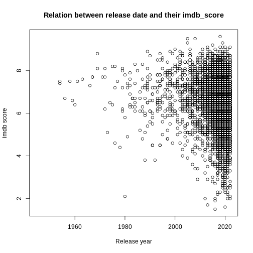
Boxplots

We can use boxplots to visualize the distribution of number of imdb_score for genre:

R

boxplot(movieSerie_plotting$imdb_score~movieSerie_plotting$genre)

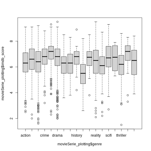
Two new things happens here. First, we are using a new way of telling the plot function what relationship we want to visualise. The function notation y~x, tells the boxplot function that we want to visualise y as a function of x. In this case we want to visualise the number of people, as af function of the wall type. Secondly, we use a boxplot. A boxplots shows the distribution of the values on the y-axis. The median value is indicated by the solid bar. The box encapsulates 50% of the observations. Its upper and lower borders represents the interquartile range (IQR). The whiskers on the plot - here only the upper whiskers are shown due to the nature of the data, represents the range of the data. The distance from the upper part of the box, to the whisker is 1.5 times the interquartile range. The dots that we see for muddaub and sunbricks are outliers. Observations that lies so far from the rest of the observations, that we consider them as outliers.

Depending on the data, and the nature of the analyses we are going to do, outliers are either very interesting, or something that we can ignore.

Histograms

Another useful plottype are histograms.

R

hist(movieSerie_plotting$runtime)

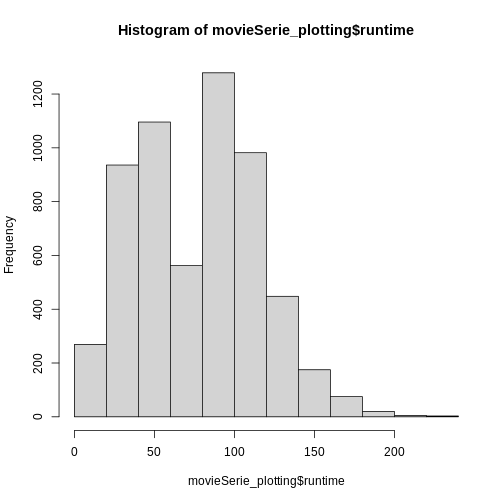
Histograms counts the number of observations in our data, that lies between two values. Here the “breaks” between the values on the x-axis corresponds nicely to the number of people, but they do not have to.

Writing our own functions

When calculating an average of several values, we do two things. First we count how many values there are. Then we sum all the values, and divides the sum by the number of values. Rather than writing R-code for each of these three operations, we use the mean() function, where other more experienced programmers have written the code.

We can write our own functions, where we collect several operations into one function.

Functions in R are defined in this way:

R

function_name <- function(x){
  temporary_result_1 <- some_function(x)
  temporary_result_2 <- some_other_function(temporary_result_1)
  yet_another_function(temporary_result_2)
}

function_name defines the name of our function.

function(x) tells R that we are defining a function, that takes X as input. We can then use that x as input to calculations or other functions within our own function.

Between the curly braces {}, we define what we want our function to do. We assign the result of some_function(x) to a temporary result, use that as the input to a second function, and the result of that as the input to a third function. The result of the last calculation we do, will be returned as the output of our function.

Exercise:

Write a function that calculates the average value of a numeric vector, takes the square root of that average, and returns the result

Show me the solution

One way to do this would be:

root_mean <- function(x){ sqrt(mean(x, na.rm=T)) }

Another way could be:

root_mean <- function(x){ temp <- mean(x, na.rm =T)> result <- sqrt(temp) result }

Logical tests in functions

Some times we want to do something different to the data, depending on the data. We can control the flow of the code using the if() construction.

As an example: if(x<10){ print(“X is smaller than 10”) }else{ print(“x is larger than 10”) }

The if() function will run the code provided in the curly braces {}, if, and only if, the expression in the paranthesis is true. If x is 11, x is not
smaller than 10, and the first print function will not be executed.

The else-part is not requiered, but normally we will have to execute some other code if the statement in the if-function is not true. In this case if x is 11, the first print-function will not be executed, but the second will.

We use logical tests to handle data differently, depending on some characteristics of the data.

loops

Loops are constructs we use to do the same operations on lots of data.

for loops

For loops are constructs used to apply one or more functions on a series of data.

R

for(i in 1:10){
  temp <- sqrt(i)
  print(temp)
}

OUTPUT

[1] 1
[1] 1.414214
[1] 1.732051
[1] 2
[1] 2.236068
[1] 2.44949
[1] 2.645751
[1] 2.828427
[1] 3
[1] 3.162278

will take every value in the vector 1:10, the digits 1 to 10, one by one, assign it to a temporary variable i and run the code we write in the curly braces. Here the for-loop will take all numbers from 1 to 10, calculate the squareroot of them. The result is assigned to another temporary variable “temp” and then temp is printed.

Danger Will Robinson

As a general rule, R does not handle loops very efficiently. This is a simple loop, operating on only 10 values, and we wont notice the difference in speed.

But we can measure it.

The Sys.time() function will tell us what time our computer thinks it is. If we run that just before, and just after our loop, we can calculate how long it took to run.

R

tic <- Sys.time()
for(i in 1:1000){
  temp <- sqrt(i)
  print(temp)
}
toc <- Sys.time()
for_time <- toc - tic

A more efficient way to calculate the square root of the numbers from 1 to 10 would be use the fact that sqrt() is a vectorized function that will calculate the square root of every element in a vector used as input to it:

R

tic <- Sys.time()
sqrt(1:1000)
toc <- Sys.time()
vect_time <- toc - tic
vect_time

And we can then compare how much faster the latter vectorized solution is.

R

as.numeric(for_time)/as.numeric(vect_time)

OUTPUT

[1] 6.605638

More than double as fast! To be fair most of the time is spent outputting the results, but as a general rule utilizing the vectorized nature of functions is faster than writing loops. But that is not always a luxury we have.

while loops

While loops are loops that execute the code - as long as some criterium is satisfied.

R

i <- 1
while(i <= 10){
  print(sqrt(i))
  i <- i + 1
}

OUTPUT

[1] 1
[1] 1.414214
[1] 1.732051
[1] 2
[1] 2.236068
[1] 2.44949
[1] 2.645751
[1] 2.828427
[1] 3
[1] 3.162278

This loop structure does the exact same as the two previous examples. Here we need to assign an initial value i, and then our while loop will execute the code within the curly braces, as long as i is smaller than or equal to 10. It is important to remember to increment the value of i - otherwise i will always be 1, and therefore always smaller than 10. And the loop will never stop.

ggplot

The plotting functions in R produce nice clean plots without any fancy details. That is generally a good thing, we want to maximize the information per ink in our plots.

However, we are limited in the types of plots we can make, and sometimes we just want a bit more color.

Enter ggplot2.

ggplot2 is a package designed to work well with the packages we have already encountered. It produces plots in a structured way, and comes with a lot of extensions, that enables us to plot almost anything.

The basic structure of ggplots are:

R

ggplot(data, mapping = aes(x=x, y=y)) +
  geom_point()

ggplot takes some data. Typically we will provide the data using the pipe: %>%

R

data %>% 
  ggplot(mapping = aes(x=x, y=y)) +
    geom_point()

The mapping argument tells ggplot which variables in our data should be mapped to the x- and y-axes in our plot.

That in itself will not produce much of a plot. We need to tell ggplot which type of plot we want.

We do that by adding a geom_ function. Here we have added geom_point which produces a scatter-plot. Other functions are more intuitively named. geom_col gives us a column-plot, geom_histogram a histogram etc.

Let us try to make a histogram like we saw earlier:

R

interviews_plotting %>% 
  ggplot(aes(x=no_membrs)) +
  geom_histogram()

ERROR

Error in eval(expr, envir, enclos): object 'interviews_plotting' not found

It looks different, and we get a warning about binwidth. geom_histogram automatically chooses 30 bins for us, and that is normally not the right number.

Key Points

Boxplots are useful for visualizing the distribution of a continuous variable.
Barplots are useful for visualizing categorical data.
Functions allows you to repeat the same set of operations again and again.
Loops allows you to apply the same function to lots of data.
Logical tests allow you to apply different calculations on different sets of data.

Content from What is the next step?

Last updated on 2024-04-30 | Edit this page