All Images
Before we Start
Figure 1

Figure 2

Figure 3
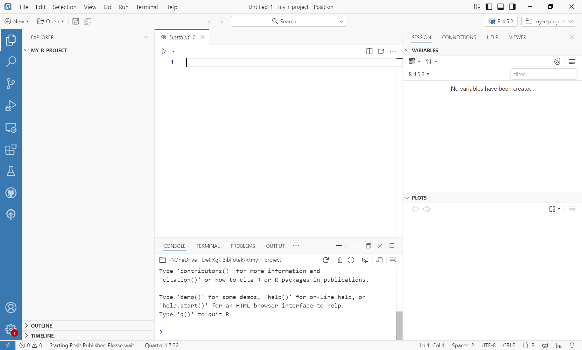
Positron interface
Figure 4
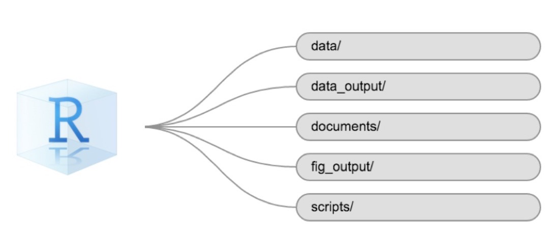
Example of a working directory structure
Introduction to R
Starting with Data
Figure 1
 {alt
= ‘A 3 by 3 data frame with columns showing numeric, character and
logical values.’}
{alt
= ‘A 3 by 3 data frame with columns showing numeric, character and
logical values.’}
Data Wrangling with dplyr and tidyr
A couple of plots. And making our own functions
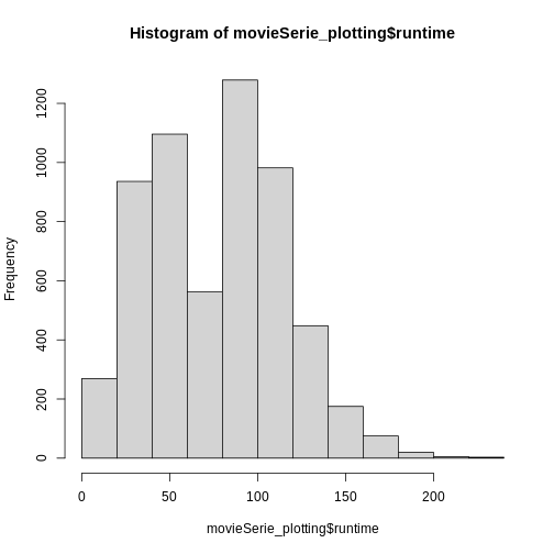
Figure 1

Figure 2
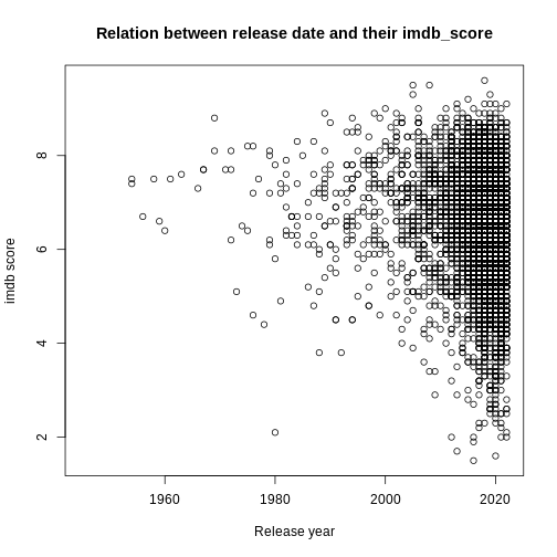
Figure 3
Figure 4