Sentiment analysis
Last updated on 2025-07-22 | Edit this page
Overview
Questions
- How is sentiment analysis conducted?
Objectives
- Learn about different lexicon
- Learn how to add sentiment to words
- Analyse and visualise the sentiments in a text
R
knitr::opts_chunk$set(warning = FALSE)
Sentiment analysis
Sentiment refers to the emotion or tone in a text. It is typically categorised as positive, negative or neutral. Sentiment is often used to analyse opinions, attitudes or emotions in written content. In this case the written content is newspaper articles.
Sentiment analysis is a method used to identify and classify emotions in textual data. This is often done using word list (lexicons). The goals is to determine whether a given text has a positive, negative or neutral tone.
In order to do a sentiment analysis on our data we From the previous section we have a dataset containing a list of words in the text without stopwords. To do a sentiment analysis we can use a so-called lexicon and assign a sentiment to each word. In order to do this we need an list of words and their sentiment. A simple form would be wether they are positive or negative.
There are multiple sentiment lexicons. For a start we will be using
the bing lexicon. This lexicon categorizes words as either
positive or negative.
R
get_sentiments("bing")
OUTPUT
# A tibble: 6,786 × 2
   word        sentiment
   <chr>       <chr>
 1 2-faces     negative
 2 abnormal    negative
 3 abolish     negative
 4 abominable  negative
 5 abominably  negative
 6 abominate   negative
 7 abomination negative
 8 abort       negative
 9 aborted     negative
10 aborts      negative
# ℹ 6,776 more rows
In order to use the bing-lexicon, we have to save
it.
R
bing <- get_sentiments("bing")
We now need to combine the sentiment to the words from our articles. We do this by performing an inner_join.
R
articles_bing <- articles_filtered %>%
  inner_join(bing)
OUTPUT
Joining with `by = join_by(word)`R
articles_bing
OUTPUT
# A tibble: 6,159 × 6
      id president web_publication_date pillar_name word          sentiment
   <dbl> <chr>     <dttm>               <chr>       <chr>         <chr>
 1     1 obama     2009-01-20 19:16:38  News        promises      positive
 2     1 obama     2009-01-20 19:16:38  News        promise       positive
 3     1 obama     2009-01-20 19:16:38  News        dust          negative
 4     1 obama     2009-01-20 19:16:38  News        cold          negative
 5     1 obama     2009-01-20 19:16:38  News        dawn          positive
 6     1 obama     2009-01-20 19:16:38  News        celebrate     positive
 7     1 obama     2009-01-20 19:16:38  News        inspirational positive
 8     1 obama     2009-01-20 19:16:38  News        failed        negative
 9     1 obama     2009-01-20 19:16:38  News        resound       positive
10     1 obama     2009-01-20 19:16:38  News        attacks       negative
# ℹ 6,149 more rows
In R, inner_join() is commonly used to combine datasets
based on a shared column. In this case it is the word
column. inner_join() matches words from a text dataset, in
this case articles_filtered with words in the Bing
sentiment lexicon to determine whether they are positive or
negative.
When we have the combined dataset we can begin making a sentiment analysis. A start could be to count the number of positive and negative words used in articles, per president.
R
articles_bing %>%
  group_by(president) %>%
  summarise(positive = sum(sentiment == "positive"),
            negative = sum(sentiment == "negative"),
            difference = positive - negative)
OUTPUT
# A tibble: 2 × 4
  president positive negative difference
  <chr>        <int>    <int>      <int>
1 obama         1499     1800       -301
2 trump         1160     1700       -540
This shows that more positive than negative words are associated with both presidents. It also shows that Trump is the president with the highest number of associated negative words.
Another interesting thing to look at would the 10 most positive and negative words used in the articles.
R
articles_bing %>%
  count(word, sentiment, sort = TRUE) %>%
  ungroup() %>%
  group_by(sentiment) %>%
  slice_max(n, n = 10) %>%
  ungroup() %>%
  mutate(word = reorder(word, n)) %>%
  ggplot(mapping = aes(n, word, fill = sentiment)) +
  geom_col(show.legend = FALSE) +
  facet_wrap(~sentiment, scales = "free_y")
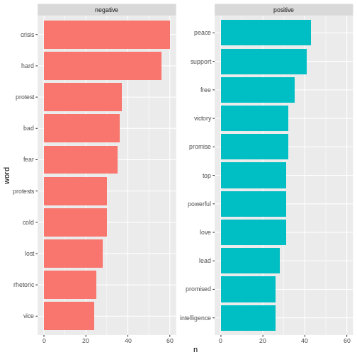 Here we can see the positive and negative words used in the
articles.
Here we can see the positive and negative words used in the
articles.
With ´bing´ we only look at the sentiment in a binary fashion - a word is either positive or negative. If we try to do a similar analysis with AFINN, it looks different.
R
install.packages("textdata")
OUTPUT
The following package(s) will be installed:
- textdata [0.4.5]
These packages will be installed into "~/work/R-textmining_new/R-textmining_new/renv/profiles/lesson-requirements/renv/library/linux-ubuntu-jammy/R-4.5/x86_64-pc-linux-gnu".

# Installing packages --------------------------------------------------------
- Installing textdata ...                       OK [linked from cache]
Successfully installed 1 package in 5.5 milliseconds.
R
library(textdata)
R
afinn <- get_sentiments("afinn")
OUTPUT
Do you want to download:
 Name: AFINN-111
 URL: http://www2.imm.dtu.dk/pubdb/views/publication_details.php?id=6010
 License: Open Database License (ODbL) v1.0
 Size: 78 KB (cleaned 59 KB)
 Download mechanism: https
ERROR
Error in menu(choices = c("Yes", "No"), title = title): menu() cannot be used non-interactivelyR
articles_afinn <- articles_filtered %>%
  inner_join(afinn)
ERROR
Error: object 'afinn' not foundR
articles_afinn %>%
  group_by(president) %>%
  summarise(sentiment = sum(value))
ERROR
Error: object 'articles_afinn' not foundR
articles_afinn %>%
  group_by(president, value) %>%
  summarise(sentiment = sum(value)) %>%
  ungroup() %>%
  ggplot(mapping = aes(x = value, y = sentiment, fill = president)) +
  geom_col(position = "dodge")
ERROR
Error: object 'articles_afinn' not foundR
articles_afinn %>%
  count(president, word, value, sort = TRUE) %>%
  ungroup() %>%
  group_by(president, value) %>%
  slice_max(n, n = 3) %>%
  ungroup() %>%
  mutate(word = reorder(word, n)) %>%
  ggplot(mapping = aes(n, word, fill = president)) +
  geom_col(show.legend = FALSE) +
  facet_wrap(~value, scales = "free_y") +
  labs(x = "Contribution to sentiment",
       y = NULL)
ERROR
Error: object 'articles_afinn' not foundKey Points
- There are different lexicons
- It is possible to add sentiments to words
- It is possible to visualise the sentiments