Content from Introduction
Last updated on 2025-07-22 | Edit this page
Overview
Questions
- What is text mining?
- What are stop words?
- What is tokenisation?
- What is tidytext?
Objectives
- Explain what text mining is
- Explain what stop words are
- Explain what tokenisation is
- Explain what tidytext is
What is text mining?
Text mining is the process of extracting meaningful information and knowledge from text. Text mining tools and methods allow the user to analyse large bodies of texts and to visualise the results.
By applying text mining principles to to a body of text, you can gain insights that would otherwise be impossible to detect with the naked eye.
Before carrying out your analysis, the text must be transformed so that it can be read by a machine.
Stopwords
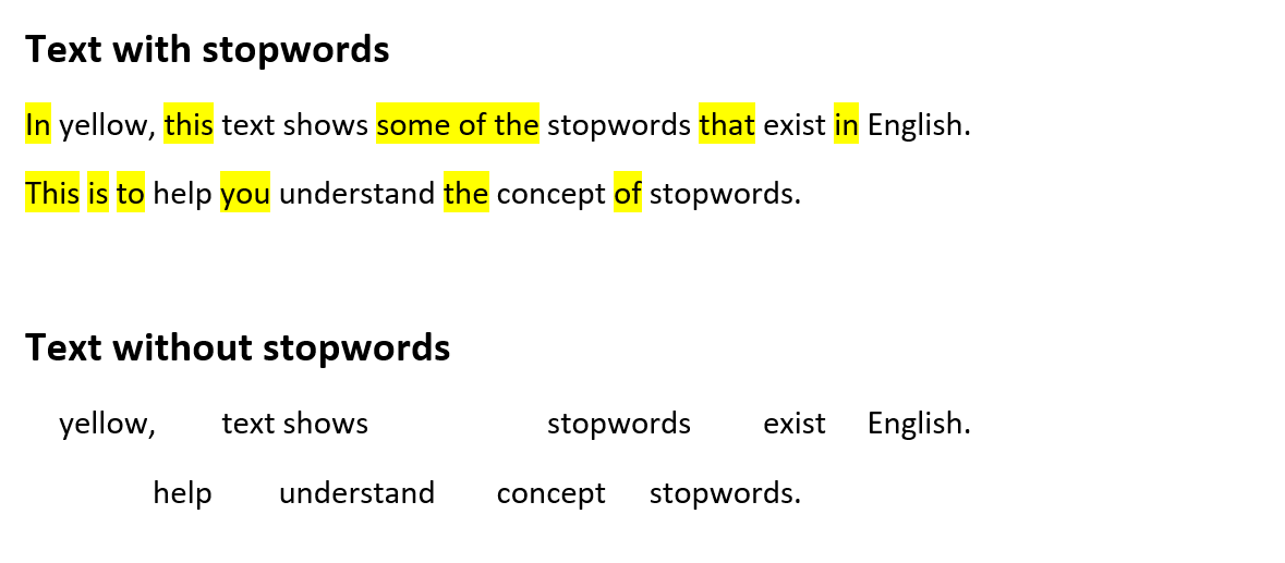
Text often contains words that hold no particular meaning. These are called stop words and can be found throughout the text. Since stop words rarely contribute to the understanding of the text, it is a good idea to remove them before analysing the text.
Example of removing stopwords
Tidytext and tokenisation
In the following we will be making the text machine-readable by means of the tidy text principles.
Tidy text
The tidy text princples were developed by Silge and Robinson (reference tilføjes - https://www.tidytextmining.com) and apply the principles from the tidy data on text.
The tidy data framework principles are:
- Each variable forms a column.
- Each observation forms a row.
- Each type of observational unit forms a table.
Applying these principles to text data leads to a format that is easily manipulated, visualised and analysed using standard data science tools.
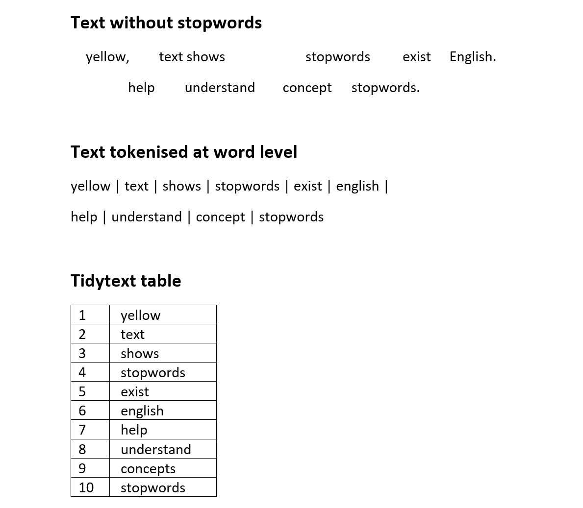
Tidy text represents the text by breaking it down into smaller parts such as sentences, words or letters. This process is called tokenisation.
Tokenisation is language independent, as long as the language uses space between each word.
Here is an example of tokenisation at word-level.
Example of tokenization
Key Points
- Know what text mining is
- Know what stop words are
- Knowledge of the data we are working with
- Know what tidy text means
Content from Loading data
Last updated on 2025-07-22 | Edit this page
Overview
Questions
- Which packages are needed?
- How is the dataset loaded?
- How is a dataset inspected?
Objectives
- Knowledge of the relevant packages
- Ability to to load the dataset
- Ability to inspect the dataset
Getting startet
When performing text analysis in R, the built-in functions in R are
not sufficient. It is therefore necessary to install some additional
packages. In this course we will be using the packages
tidyverse, tidytext and tm.
R
install.packages("tidyverse")
install.packages("tidytext")
install.packages("tm")

library(tidyverse)
library(tidytext)
library(tm)
Getting data
Begin by downloading the dataset called articles.csv.
Place the downloaded file in the data/ folder. You can do this directly
from R by copying and pasting this into your terminal. (The terminal is
the tab to the right of the console.)
R
download.file("https://raw.githubusercontent.com/KUBDatalab/R-textmining_new/main/episodes/data/articles.csv", "data/articles.csv", mode = "wb")
After downloading the data you need to load the data in R’s memory by
using the function read_csv().
R
articles <- read_csv("data/articles.csv", na = c("NA", "NULL", ""))
Data description
The dataset contains newspaper articles from the Guardian newspaper. The harvested articles were published on the first inauguration day of each of the two presidents. Inclusion criteria were that the articles contained the name of the relevant president, the word “inauguration” and a publication date similar to the inauguration date.
The original dataset contained lots of variables considered irrelevant within the parameters of this course. The following variables were kept:
- id - a unique number identifying each article
- president - the president mentioned in the article
- text - the full text from the article
- web_publication_date - the date of publication
- pillar_name - the section in the newspaper
Taking a quick look at the data
The ‘tidyverse’-package has some functions that allow you to inspect the dataset. Below, you can see some of these functions and what they do.
R
head(articles)
OUTPUT
# A tibble: 6 × 5
     id president text                          web_publication_date pillar_name
  <dbl> <chr>     <chr>                         <dttm>               <chr>
1     1 obama     "Obama inauguration: We will… 2009-01-20 19:16:38  News
2     2 obama     "Obama from outer space Whet… 2009-01-20 22:00:00  Opinion
3     3 obama     "Obama inauguration: today's… 2009-01-20 10:17:27  News
4     4 obama     "Obama inauguration: Countdo… 2009-01-19 23:01:00  News
5     5 obama     "Inaugural address of Presid… 2009-01-20 16:07:44  News
6     6 obama     "Liveblogging the inaugurati… 2009-01-20 13:56:40  News
R
tail(articles)
OUTPUT
# A tibble: 6 × 5
     id president text                          web_publication_date pillar_name
  <dbl> <chr>     <chr>                         <dttm>               <chr>
1   132 trump     Buy, George? World's largest… 2017-01-20 15:53:41  News
2   133 trump     Gove’s ‘snowflake’ tweet is … 2017-01-20 12:44:10  Opinion
3   134 trump     Monet, Renoir and a £44.2m M… 2017-01-20 04:00:22  News
4   135 trump     El Chapo is not a Robin Hood… 2017-01-20 17:09:54  News
5   136 trump     They call it fun, but the di… 2017-01-20 16:19:50  Opinion
6 137 trump Totes annoying: words that s… 2017-01-20 12:00:06 News R
glimpse(articles)
OUTPUT
Rows: 137
Columns: 5
$ id                   <dbl> 1, 2, 3, 4, 5, 6, 7, 8, 9, 10, 11, 12, 13, 14, 15…
$ president            <chr> "obama", "obama", "obama", "obama", "obama", "oba…
$ text                 <chr> "Obama inauguration: We will remake America, vows…
$ web_publication_date <dttm> 2009-01-20 19:16:38, 2009-01-20 22:00:00, 2009-0…
$ pillar_name <chr> "News", "Opinion", "News", "News", "News", "News"…R
names(articles)
OUTPUT
[1] "id"                   "president"            "text"
[4] "web_publication_date" "pillar_name" R
dim(articles)
OUTPUT
[1] 137 5Key Points
- Packages must be installed and loaded
- The dataset needs to be loaded
- The dataset can be inspected by means of different functions
Content from Tokenisation and stopwords
Last updated on 2025-07-22 | Edit this page
Overview
Questions
- How is text prepared for analysis?
Objectives
- Ability to tokenise a text
- Ability to remove stopwords from text
Tokenisation
Since we are working with text mining, we focus on the
text coloumn. We do this because the coloumn contains the
text from the articles in question.
To tokenise a coloumn, we use the functions
unnest_tokens() from the tidytext-package. The
function gets two arguments. The first one is word. This
defines that the text should be split up by words. The second argument,
text, defines the column that we want to tokenise.
R
articles_tidy <- articles %>%
  unnest_tokens(word, text)
Tokenisation
The result of the tokenisation is 118,269 rows. The reason is that
the text-column has been replaced by a new column named
word. This columns contains all words found in all of the
articles. The information from the remaining columns are kept. This
makes is possible to determine which article each word belongs to.
Stopwords
The next step is to remove stopwords. We have chosen to use the
stopword list from the package tidytext. The list contains
1,149 words that are considered stopwords. Other lists are available,
and they differ in terms of how many words they contain.
R
data(stop_words)
stop_words
OUTPUT
# A tibble: 1,149 × 2
   word        lexicon
   <chr>       <chr>
 1 a           SMART
 2 a's         SMART
 3 able        SMART
 4 about       SMART
 5 above       SMART
 6 according   SMART
 7 accordingly SMART
 8 across      SMART
 9 actually    SMART
10 after       SMART
# ℹ 1,139 more rows
Adding and removing stopwords
You may find yourself in need of either adding or removing words from the stopwords list.
Here is how you add and remove stopwords to a predefined list.
First, create a tibble with the word you wish to add to the stop words list
R
new_stop_words <- tibble(
  word = c("cat", "dog"),
  lexicon = "my_stopwords"
)
Then make a new stopwords tibble based on the original one, but with the new words added.
R
updated_stop_words <- stop_words %>%
  bind_rows(new_stop_words)
Run the following code to see that the added lexicon
my_stopwords contains two words.
R
updated_stop_words %>%
  count(lexicon)
OUTPUT
# A tibble: 4 × 2
  lexicon          n
  <chr>        <int>
1 SMART          571
2 my_stopwords     2
3 onix           404
4 snowball 174First, create a vector with the word(s) you wish to remove from the stopwords list.
R
words_to_remove <- c("cat", "dog")
Then remove the rows containing the unwanted words.
R
updated_stop_words <- stop_words %>%
  filter(!word %in% words_to_remove)
Run the following code to see that the added lexicon
my_stopwords nolonger exists.
R
updated_stop_words %>%
  count(lexicon)
OUTPUT
# A tibble: 3 × 2
lexicon n
<chr> <int>
1 SMART 571
2 onix 404
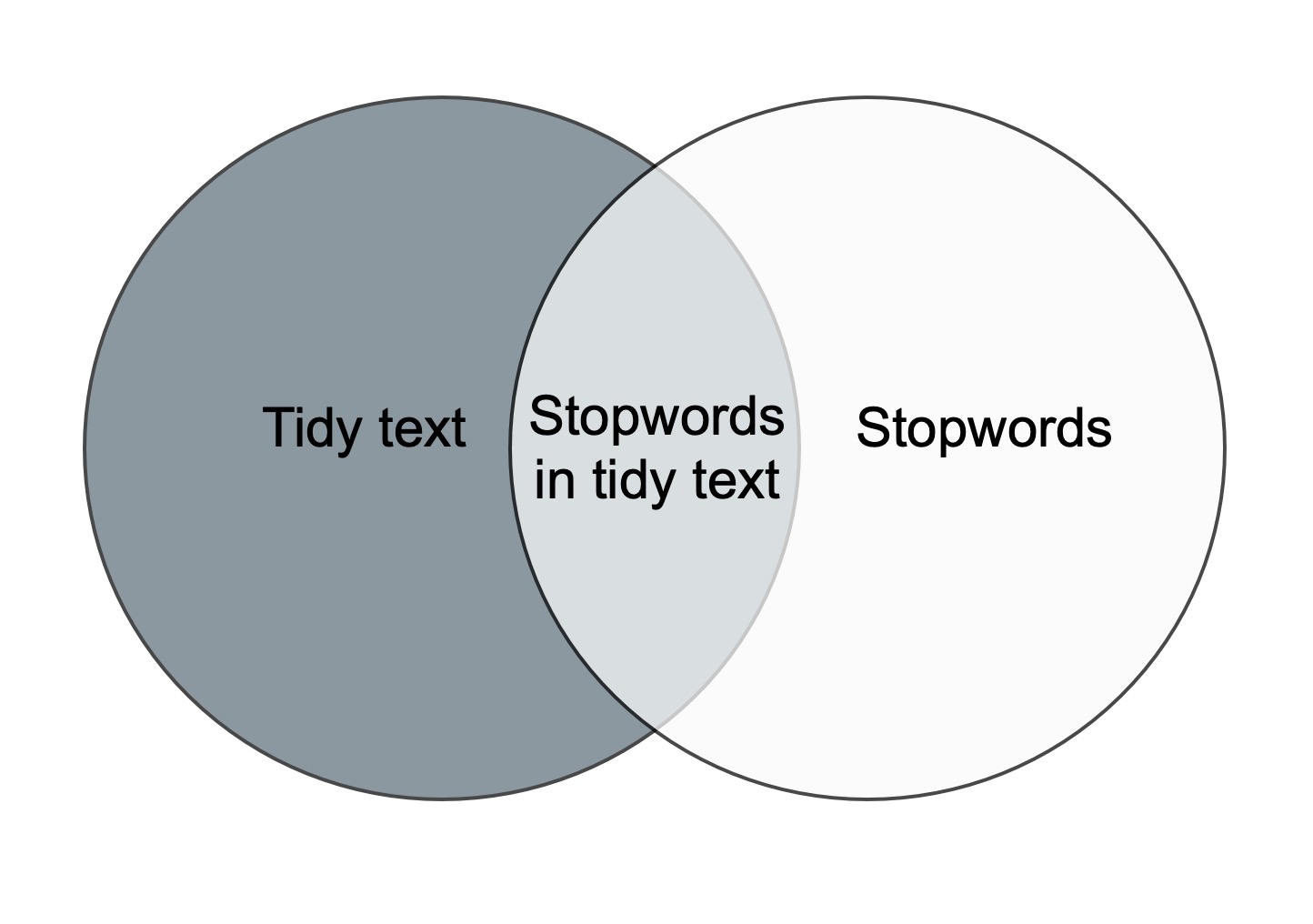
3 snowball 174In order to remove stopwords from articles_tidy, we have
to use the anti_join-function.
R
articles_anti_join <- articles_tidy %>%
  anti_join(stop_words, by = "word")
The anti_join-function removes the stopwords from the
orginal dataset. This is illustrated in the figure below. The only part
left after anti-joining is the dark grey area to the left.
These words are saved as the object
articles_anti_join.
Join and
anti_join
There are multiple join-functions in R.
Key Points
- Know how to prepare text for analysis
Content from Word frequency analysis
Last updated on 2025-07-22 | Edit this page
Overview
Questions
- How is a frequency analysis conducted?
Objectives
- Learn how to find frequent words
- Learn how to analyse and visualise it
Frequency analysis
A word frequency is a relatively simple analysis. It measures how often words occur in a text.
R
articles_anti_join %>%
  count(word, sort = TRUE)
OUTPUT
# A tibble: 12,328 × 2
   word             n
   <chr>        <int>
 1 obama          513
 2 trump          479
 3 president      450
 4 people         337
 5 inauguration   249
 6 america        237
 7 world          212
 8 american       201
 9 time           189
10 day            188
# ℹ 12,318 more rows
The previous code chunk resulted in a list containing the most frequent words. The words are from articles about both presidents, and they are sorted based on frequency with the highest number on top.
A closer look at the list may reveal that some words are irrelevant. Given that the articles in the dataset are about the two presidents’ respective inaugurations, we consider the words below irrelevant for our analysis. Therefore, we make a new dataset without these words.
R
articles_filtered <- articles_anti_join %>%
  filter(!word %in% c("trump", "trump’s", "obama", "obama's", "inauguration", "president"))

articles_filtered %>%
  count(word, sort = TRUE)
OUTPUT
# A tibble: 12,322 × 2
   word           n
   <chr>      <int>
 1 people       337
 2 america      237
 3 world        212
 4 american     201
 5 time         189
 6 day          188
 7 bush         186
 8 speech       183
 9 white        180
10 washington   150
# ℹ 12,312 more rows
The words deemed irrelevant are no longer on the list above.
Instead of a general list it may be more interesting to focus on the most frequent words belonging to articles about the two presidents respectively.
R
articles_filtered %>%
  count(president, word, sort = TRUE)
OUTPUT
# A tibble: 15,989 × 3
president word n
<chr> <chr> <int>
1 obama bush 174
2 obama people 170
3 trump people 167
4 obama america 123
5 obama speech 121
6 obama world 120
7 obama time 119
8 obama american 116
9 trump america 114
10 trump it’s 108
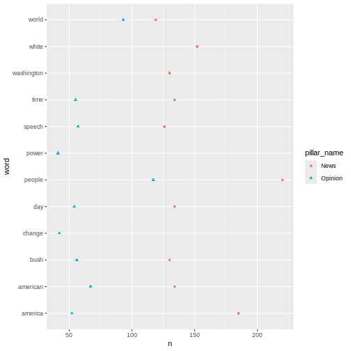
# ℹ 15,979 more rowsKeeping an overview of the words associated with each president can be a bit tricky. For instance, the word “people” is associated with both presidents. This is easy to see, as the two words are right next to each other. The two occurrences of the word America, however, are further apart, although this word is also associated with both presidents. A visualisation may solve this problem.
R
articles_filtered %>%
  count(president, word, sort = TRUE) %>%
  group_by(president) %>%
  slice(1:10) %>%
  ggplot(mapping = aes(x = n, y = word, colour = president, shape = president)) +
  geom_point()
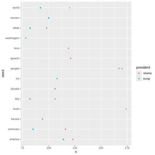 The plot above shows the top-ten words associated Obama and Trump
respectively. If a word features on both presidents’ top-ten list, it
only occurs once in the plot. This is why the plot doesn’t contain 20
words in total.
The plot above shows the top-ten words associated Obama and Trump
respectively. If a word features on both presidents’ top-ten list, it
only occurs once in the plot. This is why the plot doesn’t contain 20
words in total.
Another interesting aspect to look at would be the most frequent words used in relation to each president. In this analysis the president is the guiding principle.
R
articles_filtered %>%
  count(president, word, sort = TRUE) %>%
  pivot_wider(
    names_from = president,
    values_from = n
  )
OUTPUT
# A tibble: 12,322 × 3
   word     obama trump
   <chr>    <int> <int>
 1 bush       174    12
 2 people     170   167
 3 america    123   114
 4 speech     121    62
 5 world      120    92
 6 time       119    70
 7 american   116    85
 8 it’s        NA   108
 9 day        106    82
10 donald       1   106
# ℹ 12,312 more rows
R
articles_filtered %>%
  group_by(president) %>%
  count(word, sort = TRUE) %>%
  top_n(10) %>%
  ungroup() %>%
  mutate(word = reorder_within(word, n, president)) %>%
  ggplot(aes(n, word, fill = president)) +
  geom_col() +
  facet_wrap(~president, scales = "free") +
  scale_y_reordered() +
  labs(x = "word occurrences")
OUTPUT
Selecting by n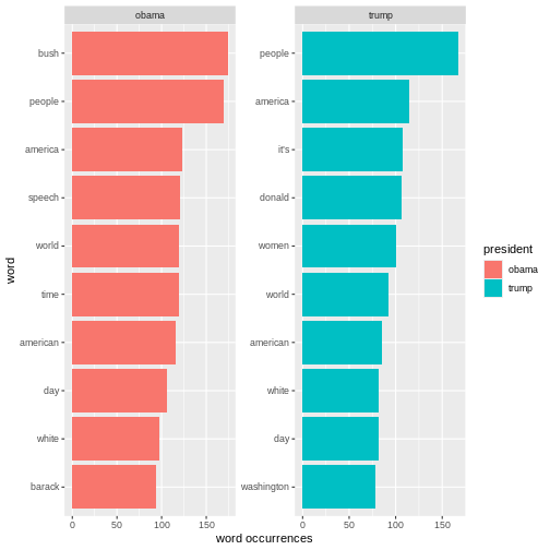 The analyses just made can easily be adjusted. For instance, if we want
look at the words by
The analyses just made can easily be adjusted. For instance, if we want
look at the words by pillar_name instead of by
president, we simply replace president with
pillar_name in the code.
R
articles_filtered %>%
  count(pillar_name, word, sort = TRUE) %>%
  group_by(pillar_name) %>%
  slice(1:10) %>%
  ggplot(mapping = aes(x = n, y = word, colour = pillar_name, shape = pillar_name)) +
  geom_point()
Key Points
- Making a frequency analysis
- Visualising the results
Content from Sentiment analysis
Last updated on 2025-07-22 | Edit this page
Overview
Questions
- How is sentiment analysis conducted?
Objectives
- Learn about different lexicon
- Learn how to add sentiment to words
- Analyse and visualise the sentiments in a text
R
knitr::opts_chunk$set(warning = FALSE)
Sentiment analysis
Sentiment refers to the emotion or tone in a text. It is typically categorised as positive, negative or neutral. Sentiment is often used to analyse opinions, attitudes or emotions in written content. In this case the written content is newspaper articles.
Sentiment analysis is a method used to identify and classify emotions in textual data. This is often done using word list (lexicons). The goals is to determine whether a given text has a positive, negative or neutral tone.
In order to do a sentiment analysis on our data we From the previous section we have a dataset containing a list of words in the text without stopwords. To do a sentiment analysis we can use a so-called lexicon and assign a sentiment to each word. In order to do this we need an list of words and their sentiment. A simple form would be wether they are positive or negative.
There are multiple sentiment lexicons. For a start we will be using
the bing lexicon. This lexicon categorizes words as either
positive or negative.
R
get_sentiments("bing")
OUTPUT
# A tibble: 6,786 × 2
   word        sentiment
   <chr>       <chr>
 1 2-faces     negative
 2 abnormal    negative
 3 abolish     negative
 4 abominable  negative
 5 abominably  negative
 6 abominate   negative
 7 abomination negative
 8 abort       negative
 9 aborted     negative
10 aborts      negative
# ℹ 6,776 more rows
In order to use the bing-lexicon, we have to save
it.
R
bing <- get_sentiments("bing")
We now need to combine the sentiment to the words from our articles. We do this by performing an inner_join.
R
articles_bing <- articles_filtered %>%
  inner_join(bing)
OUTPUT
Joining with `by = join_by(word)`R
articles_bing
OUTPUT
# A tibble: 6,159 × 6
      id president web_publication_date pillar_name word          sentiment
   <dbl> <chr>     <dttm>               <chr>       <chr>         <chr>
 1     1 obama     2009-01-20 19:16:38  News        promises      positive
 2     1 obama     2009-01-20 19:16:38  News        promise       positive
 3     1 obama     2009-01-20 19:16:38  News        dust          negative
 4     1 obama     2009-01-20 19:16:38  News        cold          negative
 5     1 obama     2009-01-20 19:16:38  News        dawn          positive
 6     1 obama     2009-01-20 19:16:38  News        celebrate     positive
 7     1 obama     2009-01-20 19:16:38  News        inspirational positive
 8     1 obama     2009-01-20 19:16:38  News        failed        negative
 9     1 obama     2009-01-20 19:16:38  News        resound       positive
10     1 obama     2009-01-20 19:16:38  News        attacks       negative
# ℹ 6,149 more rows
In R, inner_join() is commonly used to combine datasets
based on a shared column. In this case it is the word
column. inner_join() matches words from a text dataset, in
this case articles_filtered with words in the Bing
sentiment lexicon to determine whether they are positive or
negative.
When we have the combined dataset we can begin making a sentiment analysis. A start could be to count the number of positive and negative words used in articles, per president.
R
articles_bing %>%
  group_by(president) %>%
  summarise(positive = sum(sentiment == "positive"),
            negative = sum(sentiment == "negative"),
            difference = positive - negative)
OUTPUT
# A tibble: 2 × 4
  president positive negative difference
  <chr>        <int>    <int>      <int>
1 obama         1499     1800       -301
2 trump         1160     1700       -540
This shows that more positive than negative words are associated with both presidents. It also shows that Trump is the president with the highest number of associated negative words.
Another interesting thing to look at would the 10 most positive and negative words used in the articles.
R
articles_bing %>%
  count(word, sentiment, sort = TRUE) %>%
  ungroup() %>%
  group_by(sentiment) %>%
  slice_max(n, n = 10) %>%
  ungroup() %>%
  mutate(word = reorder(word, n)) %>%
  ggplot(mapping = aes(n, word, fill = sentiment)) +
  geom_col(show.legend = FALSE) +
  facet_wrap(~sentiment, scales = "free_y")
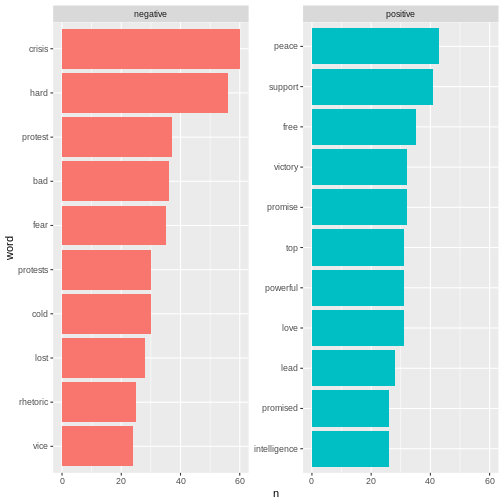 Here we can see the positive and negative words used in the
articles.
Here we can see the positive and negative words used in the
articles.
With ´bing´ we only look at the sentiment in a binary fashion - a word is either positive or negative. If we try to do a similar analysis with AFINN, it looks different.
R
install.packages("textdata")
OUTPUT
The following package(s) will be installed:
- textdata [0.4.5]
These packages will be installed into "~/work/R-textmining_new/R-textmining_new/renv/profiles/lesson-requirements/renv/library/linux-ubuntu-jammy/R-4.5/x86_64-pc-linux-gnu".

# Installing packages --------------------------------------------------------
- Installing textdata ...                       OK [linked from cache]
Successfully installed 1 package in 5.5 milliseconds.
R
library(textdata)
R
afinn <- get_sentiments("afinn")
OUTPUT
Do you want to download:
 Name: AFINN-111
 URL: http://www2.imm.dtu.dk/pubdb/views/publication_details.php?id=6010
 License: Open Database License (ODbL) v1.0
 Size: 78 KB (cleaned 59 KB)
 Download mechanism: https
ERROR
Error in menu(choices = c("Yes", "No"), title = title): menu() cannot be used non-interactivelyR
articles_afinn <- articles_filtered %>%
  inner_join(afinn)
ERROR
Error: object 'afinn' not foundR
articles_afinn %>%
  group_by(president) %>%
  summarise(sentiment = sum(value))
ERROR
Error: object 'articles_afinn' not foundR
articles_afinn %>%
  group_by(president, value) %>%
  summarise(sentiment = sum(value)) %>%
  ungroup() %>%
  ggplot(mapping = aes(x = value, y = sentiment, fill = president)) +
  geom_col(position = "dodge")
ERROR
Error: object 'articles_afinn' not foundR
articles_afinn %>%
  count(president, word, value, sort = TRUE) %>%
  ungroup() %>%
  group_by(president, value) %>%
  slice_max(n, n = 3) %>%
  ungroup() %>%
  mutate(word = reorder(word, n)) %>%
  ggplot(mapping = aes(n, word, fill = president)) +
  geom_col(show.legend = FALSE) +
  facet_wrap(~value, scales = "free_y") +
  labs(x = "Contribution to sentiment",
       y = NULL)
ERROR
Error: object 'articles_afinn' not foundKey Points
- There are different lexicons
- It is possible to add sentiments to words
- It is possible to visualise the sentiments