Before we Start
Overview
Teaching: 10 min
Exercises: 5 minQuestions
How to find your way around RStudio?
How to interact with R?
How to manage your environment?
How to install packages?
Objectives
Install latest version of R.
Install latest version of RStudio.
Navigate the RStudio GUI.
Install additional packages using the packages tab.
Install additional packages using R code.
What is R? What is RStudio?
The term “R” is used to refer to both the programming language and the
software that interprets the scripts written using it.
RStudio is currently a very popular way to not only write your R scripts but also to interact with the R software. To function correctly, RStudio needs R and therefore both need to be installed on your computer.
To make it easier to interact with R, we will use RStudio. RStudio is the most popular IDE (Integrated Development Environmemt) for R. An IDE is a piece of software that provides tools to make programming easier.
Why learn R?
R does not involve lots of pointing and clicking, and that’s a good thing
The learning curve might be steeper than with other software, but with R, the results of your analysis do not rely on remembering a succession of pointing and clicking, but instead on a series of written commands, and that’s a good thing! So, if you want to redo your analysis because you collected more data, you don’t have to remember which button you clicked in which order to obtain your results; you just have to run your script again.
Working with scripts makes the steps you used in your analysis clear, and the code you write can be inspected by someone else who can give you feedback and spot mistakes.
Working with scripts forces you to have a deeper understanding of what you are doing, and facilitates your learning and comprehension of the methods you use.
R code is great for reproducibility
Reproducibility is when someone else (including your future self) can obtain the same results from the same dataset when using the same analysis.
R integrates with other tools to generate manuscripts from your code. If you collect more data, or fix a mistake in your dataset, the figures and the statistical tests in your manuscript are updated automatically.
An increasing number of journals and funding agencies expect analyses to be reproducible, so knowing R will give you an edge with these requirements.
R is interdisciplinary and extensible
With 18,000+ packages that can be installed to extend its capabilities, R provides a framework that allows you to combine statistical approaches from many scientific disciplines to best suit the analytical framework you need to analyze your data. For instance, R has packages for image analysis, GIS, time series, population genetics, and a lot more.
R works on data of all shapes and sizes
The skills you learn with R scale easily with the size of your dataset. Whether your dataset has hundreds or millions of lines, it won’t make much difference to you.
R is designed for data analysis. It comes with special data structures and data types that make handling of missing data and statistical factors convenient.
R can connect to spreadsheets, databases, and many other data formats, on your computer or on the web.
R produces high-quality graphics
The plotting functionalities in R are endless, and allow you to adjust any aspect of your graph to convey most effectively the message from your data.
R has a large and welcoming community
Thousands of people use R daily. Many of them are willing to help you through mailing lists and websites such as Stack Overflow, or on the RStudio community. Questions which are backed up with short, reproducible code snippets are more likely to attract knowledgeable responses.
Not only is R free, but it is also open-source and cross-platform
Anyone can inspect the source code to see how R works. Because of this transparency, there is less chance for mistakes, and if you (or someone else) find some, you can report and fix bugs.
Because R is open source and is supported by a large community of developers and users, there is a very large selection of third-party add-on packages which are freely available to extend R’s native capabilities.

plot of chunk rstudio-analogy

plot of chunk rstudio-analogy-2
A tour of RStudio
Knowing your way around RStudio
Let’s start by learning about RStudio, which is an Integrated Development Environment (IDE) for working with R.
The RStudio IDE open-source product is free under the Affero General Public License (AGPL) v3. The RStudio IDE is also available with a commercial license and priority email support from RStudio, Inc.
We will use the RStudio IDE to write code, navigate the files on our computer, inspect the variables we create, and visualize the plots we generate. RStudio can also be used for other things (e.g., version control, developing packages, writing Shiny apps) that we will not cover during the workshop.
One of the advantages of using RStudio is that all the information you need to write code is available in a single window. Additionally, RStudio provides many shortcuts, autocompletion, and highlighting for the major file types you use while developing in R. RStudio makes typing easier and less error-prone.
Getting set up
It is good practice to keep a set of related data, analyses, and text self-contained in a single folder called the working directory. All of the scripts within this folder can then use relative paths to files. Relative paths indicate where inside the project a file is located (as opposed to absolute paths, which point to where a file is on a specific computer). Working this way makes it a lot easier to move your project around on your computer and share it with others without having to directly modify file paths in the individual scripts.
RStudio provides a helpful set of tools to do this through its “Projects” interface, which not only creates a working directory for you but also remembers its location (allowing you to quickly navigate to it). The interface also (optionally) preserves custom settings and open files to make it easier to resume work after a break.
Create a new project
- Under the
Filemenu, click onNew project, chooseNew directory, thenNew project - Enter a name for this new folder (or “directory”) and choose a convenient
location for it. This will be your working directory for the rest of the
day (e.g.,
~/data-carpentry) - Click on
Create project - Create a new file where we will type our scripts. Go to File > New File > R
script. Click the save icon on your toolbar and save your script as
“
script.R”.
The simplest way to open an RStudio project once it has been created is to
navigate through your files to where the project was saved and double
click on the .Rproj (blue cube) file. This will open RStudio and start your R
session in the same directory as the .Rproj file. All your data, plots and
scripts will now be relative to the project directory. RStudio projects have the
added benefit of allowing you to open multiple projects at the same time each
open to its own project directory. This allows you to keep multiple projects
open without them interfering with each other.
The RStudio Interface
Let’s take a quick tour of RStudio.
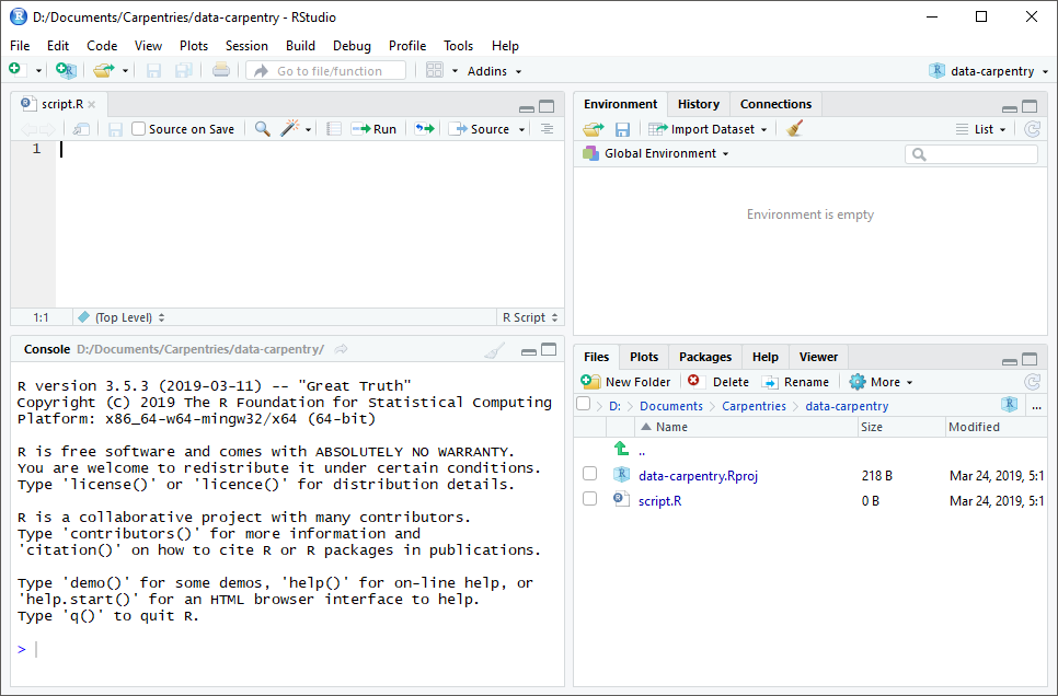
RStudio is divided into four “panes”. The placement of these panes and their content can be customized (see menu, Tools -> Global Options -> Pane Layout).
The Default Layout is:
- Top Left - Source: your scripts and documents
- Bottom Left - Console: what R would look and be like without RStudio
- Top Right - Enviornment/History: look here to see what you have done
- Bottom Right - Files and more: see the contents of the project/working directory here, like your Script.R file
Organizing your working directory
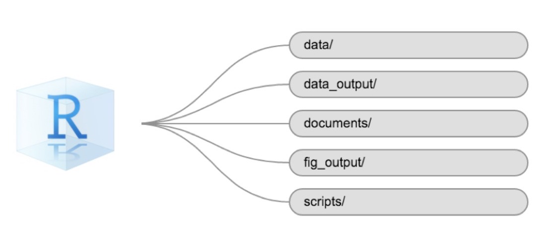
Using a consistent folder structure across your projects will help keep things organized and make it easy to find/file things in the future. This can be especially helpful when you have multiple projects. In general, you might create directories (folders) for scripts, data, and documents. Here are some examples of suggested directories:
data/Use this folder to store your raw data and intermediate datasets. For the sake of transparency and provenance, you should always keep a copy of your raw data accessible and do as much of your data cleanup and preprocessing programmatically (i.e., with scripts, rather than manually) as possible.data_output/When you need to modify your raw data, it might be useful to store the modified versions of the datasets in a different folder.documents/Used for outlines, drafts, and other text.fig_output/This folder can store the graphics that are generated by your scripts.scripts/A place to keep your R scripts for different analyses or plotting.
You may want additional directories or subdirectories depending on your project needs, but these should form the backbone of your working directory.
The working directory
The working directory is an important concept to understand. It is the place where R will look for and save files. When you write code for your project, your scripts should refer to files in relation to the root of your working directory and only to files within this structure.
Using RStudio projects makes this easy and ensures that your working directory
is set up properly. If you need to check it, you can use getwd(). If for some
reason your working directory is not the same as the location of your RStudio
project, it is likely that you opened an R script or RMarkdown file not your
.Rproj file. You should close out of RStudio and open the .Rproj file by
double clicking on the blue cube!
Downloading the data and getting set up
For this lesson we will use the following folders in our working directory:
data/, data_output/ and fig_output/. Let’s write them all in
lowercase to be consistent. We can create them using the RStudio interface by
clicking on the “New Folder” button in the file pane (bottom right), or directly
from R by typing at console:
dir.create("data")
dir.create("data_output")
dir.create("fig_output")
Begin by downloading the dataset called
“SAFI_clean.csv”. The direct download link is:
https://raw.githubusercontent.com/KUBDatalab/beginning-R/main/data/SAFI_clean.csv. Place this downloaded file in
the data/ you just created. You can do this directly from R by copying and
pasting this in your terminal (your instructor can place this chunk of code in
the Etherpad):
download.file("https://raw.githubusercontent.com/KUBDatalab/beginning-R/main/data/SAFI_clean.csv",
              "data/SAFI_clean.csv", mode = "wb")
Interacting with R
The basis of programming is that we write down instructions for the computer to follow, and then we tell the computer to follow those instructions. We write, or code, instructions in R because it is a common language that both the computer and we can understand. We call the instructions commands and we tell the computer to follow the instructions by executing (also called running) those commands.
There are two main ways of interacting with R: by using the console or by using script files (plain text files that contain your code). The console pane (in RStudio, the bottom left panel) is the place where commands written in the R language can be typed and executed immediately by the computer. It is also where the results will be shown for commands that have been executed. You can type commands directly into the console and press Enter to execute those commands, but they will be forgotten when you close the session.
Because we want our code and workflow to be reproducible, it is better to type the commands we want in the script editor and save the script. This way, there is a complete record of what we did, and anyone (including our future selves!) can easily replicate the results on their computer.
RStudio allows you to execute commands directly from the script editor by using the Ctrl + Enter shortcut (on Mac, Cmd + Return will work). The command on the current line in the script (indicated by the cursor) or all of the commands in selected text will be sent to the console and executed when you press Ctrl + Enter. If there is information in the console you do not need anymore, you can clear it with Ctrl + L. You can find other keyboard shortcuts in this RStudio cheatsheet about the RStudio IDE.
At some point in your analysis, you may want to check the content of a variable or the structure of an object without necessarily keeping a record of it in your script. You can type these commands and execute them directly in the console. RStudio provides the Ctrl + 1 and Ctrl + 2 shortcuts allow you to jump between the script and the console panes.
If R is ready to accept commands, the R console shows a > prompt. If R
receives a command (by typing, copy-pasting, or sent from the script editor using
Ctrl + Enter), R will try to execute it and, when
ready, will show the results and come back with a new > prompt to wait for new
commands.
If R is still waiting for you to enter more text,
the console will show a + prompt. It means that you haven’t finished entering
a complete command. This is likely because you have not ‘closed’ a parenthesis or
quotation, i.e. you don’t have the same number of left-parentheses as
right-parentheses or the same number of opening and closing quotation marks.
When this happens, and you thought you finished typing your command, click
inside the console window and press Esc; this will cancel the
incomplete command and return you to the > prompt. You can then proofread
the command(s) you entered and correct the error.
Installing additional packages using the packages tab
In addition to the core R installation, there are in excess of 18,000 additional packages which can be used to extend the functionality of R. Many of these have been written by R users and have been made available in central repositories, like the one hosted at CRAN, for anyone to download and install into their own R environment. You should have already installed the packages ‘ggplot2’ and ‘dplyr. If you have not, please do so now using these instructions.
You can see if you have a package installed by looking in the packages tab
(on the lower-right by default). You can also type the command
installed.packages() into the console and examine the output.
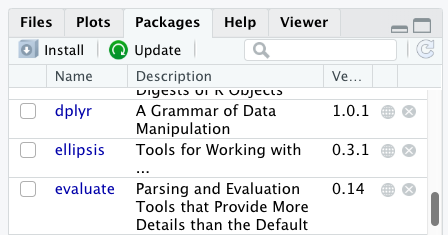
Additional packages can be installed from the ‘packages’ tab. On the packages tab, click the ‘Install’ icon and start typing the name of the package you want in the text box. As you type, packages matching your starting characters will be displayed in a drop-down list so that you can select them.
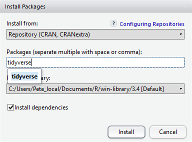
At the bottom of the Install Packages window is a check box to ‘Install’ dependencies. This is ticked by default, which is usually what you want. Packages can (and do) make use of functionality built into other packages, so for the functionality contained in the package you are installing to work properly, there may be other packages which have to be installed with them. The ‘Install dependencies’ option makes sure that this happens.
Exercise
Use both the Console and the Packages tab to confirm that you have the tidyverse installed.
Solution
Scroll through packages tab down to ‘tidyverse’. You can also type a few characters into the searchbox. The ‘tidyverse’ package is really a package of packages, including ‘ggplot2’ and ‘dplyr’, both of which require other packages to run correctly. All of these packages will be installed automatically. Depending on what packages have previously been installed in your R environment, the install of ‘tidyverse’ could be very quick or could take several minutes. As the install proceeds, messages relating to its progress will be written to the console. You will be able to see all of the packages which are actually being installed.
Because the install process accesses the CRAN repository, you will need an Internet connection to install packages.
It is also possible to install packages from other repositories, as well as Github or the local file system, but we won’t be looking at these options in this lesson.
Installing additional packages using R code
If you were watching the console window when you started the install of ‘tidyverse’, you may have noticed that the line
install.packages("tidyverse")
was written to the console before the start of the installation messages.
You could also have installed the tidyverse packages by running this command directly at the R terminal.
Key Points
Use RStudio to write and run R programs.
Use
install.packages()to install packages (libraries).
Introduction to R
Overview
Teaching: 30 min
Exercises: 10 minQuestions
What data types are available in R?
What is an object?
How can values be initially assigned to variables of different data types?
What arithmetic and logical operators can be used?
How can subsets be extracted from vectors?
How does R treat missing values?
How can we deal with missing values in R?
Objectives
Define the following terms as they relate to R: object, assign, call, function, arguments, options.
Assign values to objects in R.
Learn how to name objects.
Use comments to inform script.
Solve simple arithmetic operations in R.
Call functions and use arguments to change their default options.
Inspect the content of vectors and manipulate their content.
Subset and extract values from vectors.
Analyze vectors with missing data.
Creating objects in R
You can get output from R simply by typing math in the console:
3 + 5
[1] 8
12 / 7
[1] 1.714286
However, to do useful and interesting things, we need to assign values to
objects. To create an object, we need to give it a name followed by the
assignment operator <-, and the value we want to give it:
area_hectares <- 1.0
<- is the assignment operator. It assigns values on the right to objects on
the left. So, after executing x <- 3, the value of x is 3. The arrow can
be read as 3 goes into x. For historical reasons, you can also use =
for assignments, but not in every context. Because of the
slight
differences
in syntax, it is good practice to always use <- for assignments. More
generally we prefer the <- syntax over = because it makes it clear what
direction the assignment is operating (left assignment), and it increases the
read-ability of the code.
In RStudio, typing Alt + - (push Alt at the
same time as the - key) will write <- in a single keystroke in a
PC, while typing Option + - (push Option at the
same time as the - key) does the same in a Mac.
Objects can be given any name such as x, current_temperature, or
subject_id. You want your object names to be explicit and not too long. They
cannot start with a number (2x is not valid, but x2 is). R is case sensitive
(e.g., age is different from Age). There are some names that
cannot be used because they are the names of fundamental objects in R (e.g.,
if, else, for, see
here
for a complete list). In general, even if it’s allowed, it’s best to not use
them (e.g., c, T, mean, data, df, weights). If in
doubt, check the help to see if the name is already in use. It’s also best to
avoid dots (.) within an object name as in my.dataset. There are many
objects in R with dots in their names for historical reasons, but because dots
have a special meaning in R (for methods) and other programming languages, it’s
best to avoid them. It is also recommended to use nouns for object names, and
verbs for function names. It’s important to be consistent in the styling of your
code (where you put spaces, how you name objects, etc.). Using a consistent
coding style makes your code clearer to read for your future self and your
collaborators. In R, three popular style guides are
Google’s, Jean
Fan’s and the
tidyverse’s. The tidyverse’s is very
comprehensive and may seem overwhelming at first. You can install the
lintr package to automatically check
for issues in the styling of your code.
Objects vs. variables
What are known as
objectsinRare known asvariablesin many other programming languages. Depending on the context,objectandvariablecan have drastically different meanings. However, in this lesson, the two words are used synonymously. For more information see: https://cran.r-project.org/doc/manuals/r-release/R-lang.html#Objects
When assigning a value to an object, R does not print anything. You can force R to print the value by using parentheses or by typing the object name:
area_hectares <- 1.0    # doesn't print anything
(area_hectares <- 1.0)  # putting parenthesis around the call prints the value of `area_hectares`
[1] 1
area_hectares # and so does typing the name of the object
[1] 1
Now that R has area_hectares in memory, we can do arithmetic with it. For
instance, we may want to convert this area into acres (area in acres is 2.47 times the area in hectares):
2.47 * area_hectares
[1] 2.47
We can also change an object’s value by assigning it a new one:
area_hectares <- 2.5
2.47 * area_hectares
[1] 6.175
This means that assigning a value to one object does not change the values of
other objects. For example, let’s store the plot’s area in acres
in a new object, area_acres:
area_acres <- 2.47 * area_hectares
and then change area_hectares to 50.
area_hectares <- 50
Exercise
What do you think is the current content of the object
area_acres? 123.5 or 6.175?Solution
The value of
area_acresis still 6.175 because you have not re-run the linearea_acres <- 2.47 * area_hectaressince changing the value ofarea_hectares.
Comments
All programming languages allow the programmer to include comments in their code. To do this in R we use the # character.
Anything to the right of the # sign and up to the end of the line is treated as a comment and is ignored by R. You can start lines with comments
or include them after any code on the line.
area_hectares <- 1.0			# land area in hectares
area_acres <- area_hectares * 2.47	# convert to acres
area_acres				# print land area in acres.
[1] 2.47
RStudio makes it easy to comment or uncomment a paragraph: after selecting the lines you want to comment, press at the same time on your keyboard Ctrl + Shift + C. If you only want to comment out one line, you can put the cursor at any location of that line (i.e. no need to select the whole line), then press Ctrl + Shift + C.
Exercise
Create two variables
r_lengthandr_widthand assign them values. It should be noted that, becauselengthis a built-in R function, R Studio might add “()” after you typelengthand if you leave the parentheses you will get unexpected results. This is why you might see other programmers abbreviate common words. Create a third variabler_areaand give it a value based on the current values ofr_lengthandr_width. Show that changing the values of eitherr_lengthandr_widthdoes not affect the value ofr_area.Solution
r_length <- 2.5
r_width <- 3.2
r_area <- r_length * r_width
r_area
[1] 8# change the values of r_length and r_width r_length <- 7.0 r_width <- 6.5 # the value of r_area isn't changed r_area[1] 8
Functions and their arguments
Functions are “canned scripts” that automate more complicated sets of commands
including operations assignments, etc. Many functions are predefined, or can be
made available by importing R packages (more on that later). A function
usually gets one or more inputs called arguments. Functions often (but not
always) return a value. A typical example would be the function sqrt(). The
input (the argument) must be a number, and the return value (in fact, the
output) is the square root of that number. Executing a function (‘running it’)
is called calling the function. An example of a function call is:
b <- sqrt(a)
Here, the value of a is given to the sqrt() function, the sqrt() function
calculates the square root, and returns the value which is then assigned to
the object b. This function is very simple, because it takes just one argument.
The return ‘value’ of a function need not be numerical (like that of sqrt()),
and it also does not need to be a single item: it can be a set of things, or
even a dataset. We’ll see that when we read data files into R.
Arguments can be anything, not only numbers or filenames, but also other objects. Exactly what each argument means differs per function, and must be looked up in the documentation (see below). Some functions take arguments which may either be specified by the user, or, if left out, take on a default value: these are called options. Options are typically used to alter the way the function operates, such as whether it ignores ‘bad values’, or what symbol to use in a plot. However, if you want something specific, you can specify a value of your choice which will be used instead of the default.
Let’s try a function that can take multiple arguments: round().
round(3.14159)
[1] 3
Here, we’ve called round() with just one argument, 3.14159, and it has
returned the value 3. That’s because the default is to round to the nearest
whole number. If we want more digits we can see how to do that by getting
information about the round function. We can use args(round) or look at the
help for this function using ?round.
args(round)
function (x, digits = 0)
NULL
?round
We see that if we want a different number of digits, we can
type digits=2 or however many we want.
round(3.14159, digits = 2)
[1] 3.14
If you provide the arguments in the exact same order as they are defined you don’t have to name them:
round(3.14159, 2)
[1] 3.14
And if you do name the arguments, you can switch their order:
round(digits = 2, x = 3.14159)
[1] 3.14
It’s good practice to put the non-optional arguments (like the number you’re rounding) first in your function call, and to specify the names of all optional arguments. If you don’t, someone reading your code might have to look up the definition of a function with unfamiliar arguments to understand what you’re doing.
Exercise
Type in
?roundat the console and then look at the output in the Help pane. What other functions exist that are similar toround? How do you use thedigitsparameter in the round function?
Vectors and data types
A vector is the most common and basic data type in R, and is pretty much
the workhorse of R. A vector is composed by a series of values, which can be
either numbers or characters. We can assign a series of values to a vector using
the c() function. For example we can create a vector of the number of household
members for the households we’ve interviewed and assign
it to a new object hh_members:
hh_members <- c(3, 7, 10, 6)
hh_members
[1] 3 7 10 6
A vector can also contain characters. For example, we can have
a vector of the building material used to construct our
interview respondents’ walls (respondent_wall_type):
respondent_wall_type <- c("muddaub", "burntbricks", "sunbricks")
respondent_wall_type
[1] "muddaub" "burntbricks" "sunbricks"
The quotes around “muddaub”, etc. are essential here. Without the quotes R
will assume there are objects called muddaub, burntbricks and sunbricks. As these objects
don’t exist in R’s memory, there will be an error message.
There are many functions that allow you to inspect the content of a
vector. length() tells you how many elements are in a particular vector:
length(hh_members)
[1] 4
length(respondent_wall_type)
[1] 3
An important feature of a vector, is that all of the elements are the same type of data.
The function class() indicates the class (the type of element) of an object:
class(hh_members)
[1] "numeric"
class(respondent_wall_type)
[1] "character"
The function str() provides an overview of the structure of an object and its
elements. It is a useful function when working with large and complex
objects:
str(hh_members)
num [1:4] 3 7 10 6
str(respondent_wall_type)
chr [1:3] "muddaub" "burntbricks" "sunbricks"
You can use the c() function to add other elements to your vector:
possessions <- c("bicycle", "radio", "television")
possessions <- c(possessions, "mobile_phone") # add to the end of the vector
possessions <- c("car", possessions) # add to the beginning of the vector
possessions
[1] "car" "bicycle" "radio" "television" "mobile_phone"
In the first line, we take the original vector possessions,
add the value "mobile_phone" to the end of it, and save the result back into
possessions. Then we add the value "car" to the beginning, again saving the result
back into possessions.
We can do this over and over again to grow a vector, or assemble a dataset. As we program, this may be useful to add results that we are collecting or calculating.
An atomic vector is the simplest R data type and is a linear vector of a single type. Above, we saw
2 of the 6 main atomic vector types that R
uses: "character" and "numeric" (or "double"). These are the basic building blocks that
all R objects are built from. The other 4 atomic vector types are:
"logical"forTRUEandFALSE(the boolean data type)"integer"for integer numbers (e.g.,2L, theLindicates to R that it’s an integer)"complex"to represent complex numbers with real and imaginary parts (e.g.,1 + 4i) and that’s all we’re going to say about them"raw"for bitstreams that we won’t discuss further
You can check the type of your vector using the typeof() function and inputting your vector as the argument.
Vectors are one of the many data structures that R uses. Other important
ones are lists (list), matrices (matrix), data frames (data.frame),
factors (factor) and arrays (array).
Exercise
We’ve seen that atomic vectors can be of type character, numeric (or double), integer, and logical. But what happens if we try to mix these types in a single vector?
Solution
R implicitly converts them to all be the same type.
What will happen in each of these examples? (hint: use
class()to check the data type of your objects):num_char <- c(1, 2, 3, "a") num_logical <- c(1, 2, 3, TRUE) char_logical <- c("a", "b", "c", TRUE) tricky <- c(1, 2, 3, "4")Why do you think it happens?
Solution
Vectors can be of only one data type. R tries to convert (coerce) the content of this vector to find a “common denominator” that doesn’t lose any information.
How many values in
combined_logicalare"TRUE"(as a character) in the following example:num_logical <- c(1, 2, 3, TRUE) char_logical <- c("a", "b", "c", TRUE) combined_logical <- c(num_logical, char_logical)
Solution
Only one. There is no memory of past data types, and the coercion happens the first time the vector is evaluated. Therefore, the
TRUEinnum_logicalgets converted into a1before it gets converted into"1"incombined_logical.You’ve probably noticed that objects of different types get converted into a single, shared type within a vector. In R, we call converting objects from one class into another class coercion. These conversions happen according to a hierarchy, whereby some types get preferentially coerced into other types. Can you draw a diagram that represents the hierarchy of how these data types are coerced?
Subsetting vectors
If we want to extract one or several values from a vector, we must provide one or several indices in square brackets. For instance:
respondent_wall_type <- c("muddaub", "burntbricks", "sunbricks")
respondent_wall_type[2]
[1] "burntbricks"
respondent_wall_type[c(3, 2)]
[1] "sunbricks" "burntbricks"
We can also repeat the indices to create an object with more elements than the original one:
more_respondent_wall_type <- respondent_wall_type[c(1, 2, 3, 2, 1, 3)]
more_respondent_wall_type
[1] "muddaub"     "burntbricks" "sunbricks"   "burntbricks" "muddaub"
[6] "sunbricks"
R indices start at 1. Programming languages like Fortran, MATLAB, Julia, and R start counting at 1, because that’s what human beings typically do. Languages in the C family (including C++, Java, Perl, and Python) count from 0 because that’s simpler for computers to do.
Conditional subsetting
Another common way of subsetting is by using a logical vector. TRUE will
select the element with the same index, while FALSE will not:
hh_members <- c(3, 7, 10, 6)
hh_members[c(TRUE, FALSE, TRUE, TRUE)]
[1] 3 10 6
Typically, these logical vectors are not typed by hand, but are the output of other functions or logical tests. For instance, if you wanted to select only the values above 5:
hh_members > 5 # will return logicals with TRUE for the indices that meet the condition
[1] FALSE TRUE TRUE TRUE
## so we can use this to select only the values above 5
hh_members[hh_members > 5]
[1] 7 10 6
You can combine multiple tests using & (both conditions are true, AND) or |
(at least one of the conditions is true, OR):
hh_members[hh_members < 4 | hh_members > 7]
[1] 3 10
hh_members[hh_members >= 4 & hh_members <= 7]
[1] 7 6
Here, < stands for “less than”, > for “greater than”, >= for “greater than
or equal to”, and == for “equal to”. The double equal sign == is a test for
numerical equality between the left and right hand sides, and should not be
confused with the single = sign, which performs variable assignment (similar
to <-).
A common task is to search for certain strings in a vector. One could use the
“or” operator | to test for equality to multiple values, but this can quickly
become tedious.
possessions <- c("car", "bicycle", "radio", "television", "mobile_phone")
possessions[possessions == "car" | possessions == "bicycle"] # returns both car and bicycle
[1] "car" "bicycle"
The function %in% allows you to test if any of the elements of a search vector
(on the left hand side) are found in the target vector (on the right hand side):
possessions %in% c("car", "bicycle")
[1] TRUE TRUE FALSE FALSE FALSE
Note that the output is the same length as the search vector on the left hand
side, because %in% checks whether each element of the search vector is found
somewhere in the target vector. Thus, you can use %in% to select the elements
in the search vector that appear in your target vector:
possessions %in% c("car", "bicycle", "motorcycle", "truck", "boat", "bus")
[1] TRUE TRUE FALSE FALSE FALSE
possessions[possessions %in% c("car", "bicycle", "motorcycle", "truck", "boat", "bus")]
[1] "car" "bicycle"
Missing data
As R was designed to analyze datasets, it includes the concept of missing data
(which is uncommon in other programming languages). Missing data are represented
in vectors as NA.
When doing operations on numbers, most functions will return NA if the data
you are working with include missing values. This feature
makes it harder to overlook the cases where you are dealing with missing data.
You can add the argument na.rm=TRUE to calculate the result while ignoring
the missing values.
rooms <- c(2, 1, 1, NA, 7)
mean(rooms)
[1] NA
max(rooms)
[1] NA
mean(rooms, na.rm = TRUE)
[1] 2.75
max(rooms, na.rm = TRUE)
[1] 7
If your data include missing values, you may want to become familiar with the
functions is.na(), na.omit(), and complete.cases(). See below for
examples.
## Extract those elements which are not missing values.
rooms[!is.na(rooms)]
[1] 2 1 1 7
## Count the number of missing values.
sum(is.na(rooms))
[1] 1
## Returns the object with incomplete cases removed. The returned object is an atomic vector of type `"numeric"` (or `"double"`).
na.omit(rooms)
[1] 2 1 1 7
attr(,"na.action")
[1] 4
attr(,"class")
[1] "omit"
## Extract those elements which are complete cases. The returned object is an atomic vector of type `"numeric"` (or `"double"`).
rooms[complete.cases(rooms)]
[1] 2 1 1 7
Recall that you can use the typeof() function to find the type of your atomic vector.
Exercise
Using this vector of rooms, create a new vector with the NAs removed.
rooms <- c(1, 2, 1, 1, NA, 3, 1, 3, 2, 1, 1, 8, 3, 1, NA, 1)Use the function
median()to calculate the median of theroomsvector.Use R to figure out how many households in the set use more than 2 rooms for sleeping.
Solution
rooms <- c(1, 2, 1, 1, NA, 3, 1, 3, 2, 1, 1, 8, 3, 1, NA, 1)
rooms_no_na <- rooms[!is.na(rooms)]
# or
rooms_no_na <- na.omit(rooms)
# 2.
median(rooms, na.rm = TRUE)
[1] 1# 3. rooms_above_2 <- rooms_no_na[rooms_no_na > 2] length(rooms_above_2)[1] 4
Now that we have learned how to write scripts, and the basics of R’s data structures, we are ready to start working a real dataset, and learn about data frames.
Key Points
Access individual values by location using
[].Access arbitrary sets of data using
[c(...)].Use logical operations and logical vectors to access subsets of data.
Starting with Data
Overview
Teaching: 30 min
Exercises: 10 minQuestions
What is a data.frame?
How can I read a complete csv file into R?
How can I get basic summary information about my dataset?
Objectives
Describe what a data frame is.
Load external data from a .csv file into a data frame.
Summarize the contents of a data frame.
Subset and extract values from data frames.
What are data frames and tibbles?
Data frames are the de facto data structure for tabular data in R, and what
we use for data processing, statistics, and plotting.
A data frame is the representation of data in the format of a table where the columns are vectors that all have the same length. Data frames are analogous to the more familiar spreadsheet in programs such as Excel, with one key difference. Because columns are vectors, each column must contain a single type of data (e.g., characters, integers, factors). For example, here is a figure depicting a data frame comprising a numeric, a character, and a logical vector.

Data frames can be created by hand, but most commonly they are generated by the
functions read_csv() or read_table(); in other words, when importing
spreadsheets from your hard drive (or the web). We will now demonstrate how to
import tabular data using read_csv().
Presentation of the SAFI Data
SAFI (Studying African Farmer-Led Irrigation) is a study looking at farming and irrigation methods in Tanzania and Mozambique. The survey data was collected through interviews conducted between November 2016 and June 2017. For this lesson, we will be using a subset of the available data. For information about the full dataset, see the dataset description.
We will be using a subset of the cleaned version of the dataset that
was produced through cleaning in OpenRefine (data/SAFI_clean.csv). Each row holds
information for a single interview respondent, and the columns
represent:
| column_name | description |
|---|---|
| key_id | Added to provide a unique Id for each observation. (The InstanceID field does this as well but it is not as convenient to use) |
| village | Village name |
| interview_date | Date of interview |
| no_membrs | How many members in the household? |
| respondent_wall_type | What type of walls does their house have (from list) |
| no_meals | How many meals do people in your household normally eat in a day? |
Importing data
You are going load the data in R’s memory using the function read_csv()
from the readr package, which is part of the tidyverse; learn
more about the tidyverse collection of packages
here.
readr gets installed as part as the tidyverse installation.
When you load the tidyverse (library(tidyverse)), the core packages
(the packages used in most data analyses) get loaded, including readr.
Before we can use the read_csv() we need to load the tidyverse package.
Also, if you recall, the missing data is encoded as “NULL” in the dataset.
We’ll tell it to the function, so R will automatically convert all the “NULL”
entries in the dataset into NA.
The specific path we are using here is dependent on the specific setup. If you have followed the recommendations for structuring your project-folder, it should be this command:
library(tidyverse)

interviews <- read_csv("data/SAFI_clean.csv", na = "NULL")
If you were to type in the code above, it is likely that the read.csv()
function would appear in the automatically populated list of functions. This
function is different from the read_csv() function, as it is included in the
“base” packages that come pre-installed with R. Overall, read.csv() behaves
similar to read_csv(), with a few notable differences. First, read.csv()
coerces column names with spaces and/or special characters to different names
(e.g. interview date becomes interview.date). Second, read.csv()
stores data as a data.frame, where read_csv() stores data as a tibble.
We prefer tibbles because they have nice printing properties among other
desirable qualities. Read more about tibbles
here.
The second statement in the code above creates a data frame but doesn’t output
any data because, as you might recall, assignments (<-) don’t display
anything. (Note, however, that read_csv may show informational
text about the data frame that is created.) If we want to check that our data
has been loaded, we can see the contents of the data frame by typing its name:
interviews in the console.
interviews
## Try also
## view(interviews)
## head(interviews)
# A tibble: 131 × 6
   key_ID village  interview_date      no_membrs respondent_wall_type no_meals
    <dbl> <chr>    <dttm>                  <dbl> <chr>                   <dbl>
 1      1 God      2016-11-17 00:00:00         3 muddaub                     2
 2      1 God      2016-11-17 00:00:00         7 muddaub                     2
 3      3 God      2016-11-17 00:00:00        10 burntbricks                 2
 4      4 God      2016-11-17 00:00:00         7 burntbricks                 2
 5      5 God      2016-11-17 00:00:00         7 burntbricks                 2
 6      6 God      2016-11-17 00:00:00         3 muddaub                     2
 7      7 God      2016-11-17 00:00:00         6 muddaub                     3
 8      8 Chirodzo 2016-11-16 00:00:00        12 burntbricks                 2
 9      9 Chirodzo 2016-11-16 00:00:00         8 burntbricks                 3
10     10 Chirodzo 2016-12-16 00:00:00        12 burntbricks                 3
# ℹ 121 more rows
Note
read_csv()assumes that fields are delimited by commas. However, in several countries, the comma is used as a decimal separator and the semicolon (;) is used as a field delimiter. If you want to read in this type of files in R, you can use theread_csv2function. It behaves exactly likeread_csvbut uses different parameters for the decimal and the field separators. If you are working with another format, they can be both specified by the user. Check out the help forread_csv()by typing?read_csvto learn more. There is also theread_tsv()for tab-separated data files, andread_delim()allows you to specify more details about the structure of your file.
Note that read_csv() actually loads the data as a tibble.
A tibble is an extension of R data frames used by the tidyverse. When
the data is read using read_csv(), it is stored in an object of class
tbl_df, tbl, and data.frame. You can see the class of an object with
class(interviews)
[1] "spec_tbl_df" "tbl_df" "tbl" "data.frame"
As a tibble, the type of data included in each column is listed in an
abbreviated fashion below the column names. For instance, here key_ID is a
column of floating point numbers (abbreviated <dbl> for the word ‘double’),
village is a column of characters (<chr>) and the interview_date is a
column in the “date and time” format (<dttm>).
Inspecting data frames
When calling a tbl_df object (like interviews here), there is already a lot
of information about our data frame being displayed such as the number of rows,
the number of columns, the names of the columns, and as we just saw the class of
data stored in each column. However, there are functions to extract this
information from data frames. Here is a non-exhaustive list of some of these
functions. Let’s try them out!
Size:
dim(interviews)- returns a vector with the number of rows as the first element, and the number of columns as the second element (the dimensions of the object)nrow(interviews)- returns the number of rowsncol(interviews)- returns the number of columns
Content:
head(interviews)- shows the first 6 rowstail(interviews)- shows the last 6 rows
Names:
names(interviews)- returns the column names (synonym ofcolnames()fordata.frameobjects)
Summary:
str(interviews)- structure of the object and information about the class, length and content of each columnsummary(interviews)- summary statistics for each columnglimpse(interviews)- returns the number of columns and rows of the tibble, the names and class of each column, and previews as many values will fit on the screen. Unlike the other inspecting functions listed above,glimpse()is not a “base R” function so you need to have thedplyrortibblepackages loaded to be able to execute it.
Note: most of these functions are “generic.” They can be used on other types of objects besides data frames or tibbles.
Indexing and subsetting data frames
Our interviews data frame has rows and columns (it has 2 dimensions).
In practice, we may not need the entire data frame; for instance, we may only
be interested in a subset of the observations (the rows) or a particular set
of variables (the columns). If we want to
extract some specific data from it, we need to specify the “coordinates” we
want from it. Row numbers come first, followed by column numbers.
Tip
Indexing a
tibblewith[or[[or$always results in atibble. However, note this is not true in general for data frames, so be careful! Different ways of specifying these coordinates can lead to results with different classes. This is covered in the Software Carpentry lesson R for Reproducible Scientific Analysis.
## first element in the first column of the tibble
interviews[1, 1]
# A tibble: 1 × 1
  key_ID
   <dbl>
1      1
## first element in the 6th column of the tibble
interviews[1, 6]
# A tibble: 1 × 1
  no_meals
     <dbl>
1        2
## first column of the tibble (as a vector)
interviews[[1]]
  [1]   1   1   3   4   5   6   7   8   9  10  11  12  13  14  15  16  17  18
 [19]  19  20  21  22  23  24  25  26  27  28  29  30  31  32  33  34  35  36
 [37]  37  38  39  40  41  42  43  44  45  46  47  48  49  50  51  52  21  54
 [55]  55  56  57  58  59  60  61  62  63  64  65  66  67  68  69  70  71 127
 [73] 133 152 153 155 178 177 180 181 182 186 187 195 196 197 198 201 202  72
 [91]  73  76  83  85  89 101 103 102  78  80 104 105 106 109 110 113 118 125
[109] 119 115 108 116 117 144 143 150 159 160 165 166 167 174 175 189 191 192
[127] 126 193 194 199 200
## first column of the tibble
interviews[1]
# A tibble: 131 × 1
   key_ID
    <dbl>
 1      1
 2      1
 3      3
 4      4
 5      5
 6      6
 7      7
 8      8
 9      9
10     10
# ℹ 121 more rows
## first three elements in the 7th column of the tibble
interviews[1:3, 7]
Error in `interviews[1:3, 7]`:
! Can't subset columns past the end.
ℹ Location 7 doesn't exist.
ℹ There are only 6 columns.
## the 3rd row of the tibble
interviews[3, ]
# A tibble: 1 × 6
  key_ID village interview_date      no_membrs respondent_wall_type no_meals
   <dbl> <chr>   <dttm>                  <dbl> <chr>                   <dbl>
1      3 God     2016-11-17 00:00:00        10 burntbricks                 2
## equivalent to head_interviews <- head(interviews)
head_interviews <- interviews[1:6, ]
: is a special function that creates numeric vectors of integers in increasing
or decreasing order, test 1:10 and 10:1 for instance.
You can also exclude certain indices of a data frame using the “-” sign:
interviews[, -1] # The whole tibble, except the first column
# A tibble: 131 × 5
   village  interview_date      no_membrs respondent_wall_type no_meals
   <chr>    <dttm>                  <dbl> <chr>                   <dbl>
 1 God      2016-11-17 00:00:00         3 muddaub                     2
 2 God      2016-11-17 00:00:00         7 muddaub                     2
 3 God      2016-11-17 00:00:00        10 burntbricks                 2
 4 God      2016-11-17 00:00:00         7 burntbricks                 2
 5 God      2016-11-17 00:00:00         7 burntbricks                 2
 6 God      2016-11-17 00:00:00         3 muddaub                     2
 7 God      2016-11-17 00:00:00         6 muddaub                     3
 8 Chirodzo 2016-11-16 00:00:00        12 burntbricks                 2
 9 Chirodzo 2016-11-16 00:00:00         8 burntbricks                 3
10 Chirodzo 2016-12-16 00:00:00        12 burntbricks                 3
# ℹ 121 more rows
interviews[-c(7:131), ] # Equivalent to head(interviews)
# A tibble: 6 × 6
  key_ID village interview_date      no_membrs respondent_wall_type no_meals
   <dbl> <chr>   <dttm>                  <dbl> <chr>                   <dbl>
1      1 God     2016-11-17 00:00:00         3 muddaub                     2
2      1 God     2016-11-17 00:00:00         7 muddaub                     2
3      3 God     2016-11-17 00:00:00        10 burntbricks                 2
4      4 God     2016-11-17 00:00:00         7 burntbricks                 2
5      5 God     2016-11-17 00:00:00         7 burntbricks                 2
6      6 God     2016-11-17 00:00:00         3 muddaub                     2
tibbles can be subset by calling indices (as shown previously), but also by
calling their column names directly:
interviews["village"]       # Result is a tibble

interviews[, "village"]     # Result is a tibble

interviews[["village"]]     # Result is a vector

interviews$village          # Result is a vector
In RStudio, you can use the autocompletion feature to get the full and correct names of the columns.
Exercise
Create a tibble (
interviews_100) containing only the data in row 100 of theinterviewsdataset.Notice how
nrow()gave you the number of rows in the tibble?
- Use that number to pull out just that last row in the tibble.
- Compare that with what you see as the last row using
tail()to make sure it’s meeting expectations.- Pull out that last row using
nrow()instead of the row number.- Create a new tibble (
interviews_last) from that last row.Using the number of rows in the interviews dataset that you found in question 2, extract the row that is in the middle of the dataset. Store the content of this middle row in an object named
interviews_middle. (hint: This dataset has an odd number of rows, so finding the middle is a bit trickier than dividing n_rows by 2. Use the median( ) function and what you’ve learned about sequences in R to extract the middle row!Combine
nrow()with the-notation above to reproduce the behavior ofhead(interviews), keeping just the first through 6th rows of the interviews dataset.Solution
## 1.
interviews_100 <- interviews[100, ]
## 2.
# Saving `n_rows` to improve readability and reduce duplication
n_rows <- nrow(interviews)
interviews_last <- interviews[n_rows, ]
## 3.
interviews_middle <- interviews[median(1:n_rows), ]
## 4.
interviews_head <- interviews[-(7:n_rows), ]
Key Points
Use read_csv to read tabular data in R.
Data Wrangling with dplyr and tidyr
Overview
Teaching: 20 min
Exercises: 10 minQuestions
How can I select specific rows and/or columns from a dataframe?
How can I combine multiple commands into a single command?
How can I create new columns or remove existing columns from a dataframe?
How can I reformat a dataframe to meet my needs?
Objectives
Describe the purpose of an R package and the
dplyrandtidyrpackages.Select certain columns in a dataframe with the
dplyrfunctionselect.Select certain rows in a dataframe according to filtering conditions with the
dplyrfunctionfilter.Link the output of one
dplyrfunction to the input of another function with the ‘pipe’ operator%>%.Add new columns to a dataframe that are functions of existing columns with
mutate.Use the split-apply-combine concept for data analysis.
Use
summarize,group_by, andcountto split a dataframe into groups of observations, apply a summary statistics for each group, and then combine the results.Describe the concept of a wide and a long table format and for which purpose those formats are useful.
Describe the roles of variable names and their associated values when a table is reshaped.
Reshape a dataframe from long to wide format and back with the
pivot_widerandpivot_longercommands from thetidyrpackage.Export a dataframe to a csv file.
dplyr is a package for making tabular data wrangling easier by using a
limited set of functions that can be combined to extract and summarize insights
from your data. It pairs nicely with tidyr which enables you to swiftly
convert between different data formats (long vs. wide) for plotting and analysis.
Similarly to readr, dplyr and tidyr are also part of the
tidyverse. These packages were loaded in R’s memory when we called
library(tidyverse) earlier.
Note
The packages in the tidyverse, namely
dplyr,tidyrandggplot2accept both the British (e.g. summarise) and American (e.g. summarize) spelling variants of different function and option names. For this lesson, we utilize the American spellings of different functions; however, feel free to use the regional variant for where you are teaching.
What is an R package?
The package dplyr provides easy tools for the most common data
wrangling tasks. It is built to work directly with dataframes, with many
common tasks optimized by being written in a compiled language (C++) (not all R
packages are written in R!).
The package tidyr addresses the common problem of wanting to reshape your
data for plotting and use by different R functions. Sometimes we want data sets
where we have one row per measurement. Sometimes we want a dataframe where each
measurement type has its own column, and rows are instead more aggregated
groups. Moving back and forth between these formats is nontrivial, and
tidyr gives you tools for this and more sophisticated data wrangling.
But there are also packages available for a wide range of tasks including
building plots (ggplot2, which we’ll see later), downloading data from the
NCBI database, or performing statistical analysis on your data set. Many
packages such as these are housed on, and downloadable from, the
Comprehensive R Archive Network (CRAN) using install.packages.
This function makes the package accessible by your R installation with the
command library(), as you did with tidyverse earlier.
To easily access the documentation for a package within R or RStudio, use
help(package = "package_name").
To learn more about dplyr and tidyr after the workshop, you may want
to check out this handy data transformation with dplyr cheatsheet
and this one about tidyr.
Learning dplyr and tidyr
We are working with the same dataset as earlier. Refer to the previous lesson to download the data, if you do not have it loaded.
We’re going to learn some of the most common dplyr functions:
select(): subset columnsfilter(): subset rows on conditionsmutate(): create new columns by using information from other columnsgroup_by()andsummarize(): create summary statistics on grouped dataarrange(): sort resultscount(): count discrete values
Selecting columns and filtering rows
To select columns of a dataframe, use select(). The first argument to this
function is the dataframe (interviews), and the subsequent arguments are the
columns to keep, separated by commas. Alternatively, if you are selecting
columns adjacent to each other, you can use a : to select a range of columns,
read as “select columns from __ to __.”
# to select columns throughout the dataframe
select(interviews, village, no_membrs)
# to select a series of connected columns
select(interviews, village:respondent_wall_type)
To choose rows based on specific criteria, we can use the filter() function.
The argument after the dataframe is the condition we want our final
dataframe to adhere to (e.g. village name is Chirodzo):
# filters observations where village name is "Chirodzo"
filter(interviews, village == "Chirodzo")
# A tibble: 39 × 6
   key_ID village  interview_date      no_membrs respondent_wall_type no_meals
    <dbl> <chr>    <dttm>                  <dbl> <chr>                   <dbl>
 1      8 Chirodzo 2016-11-16 00:00:00        12 burntbricks                 2
 2      9 Chirodzo 2016-11-16 00:00:00         8 burntbricks                 3
 3     10 Chirodzo 2016-12-16 00:00:00        12 burntbricks                 3
 4     34 Chirodzo 2016-11-17 00:00:00         8 burntbricks                 2
 5     35 Chirodzo 2016-11-17 00:00:00         5 muddaub                     3
 6     36 Chirodzo 2016-11-17 00:00:00         6 sunbricks                   3
 7     37 Chirodzo 2016-11-17 00:00:00         3 burntbricks                 3
 8     43 Chirodzo 2016-11-17 00:00:00         7 muddaub                     2
 9     44 Chirodzo 2016-11-17 00:00:00         2 muddaub                     2
10     45 Chirodzo 2016-11-17 00:00:00         9 muddaub                     3
# ℹ 29 more rows
We can also specify multiple conditions within the filter() function. We can
combine conditions using either “and” or “or” statements. In an “and”
statement, an observation (row) must meet every criteria to be included
in the resulting dataframe. To form “and” statements within dplyr, we can pass
our desired conditions as arguments in the filter() function, separated by
commas:
# filters observations with "and" operator (comma)
# output dataframe satisfies ALL specified conditions
filter(interviews, village == "Chirodzo",
                   no_membrs > 4,
                   no_meals > 2)
# A tibble: 20 × 6
   key_ID village  interview_date      no_membrs respondent_wall_type no_meals
    <dbl> <chr>    <dttm>                  <dbl> <chr>                   <dbl>
 1      9 Chirodzo 2016-11-16 00:00:00         8 burntbricks                 3
 2     10 Chirodzo 2016-12-16 00:00:00        12 burntbricks                 3
 3     35 Chirodzo 2016-11-17 00:00:00         5 muddaub                     3
 4     36 Chirodzo 2016-11-17 00:00:00         6 sunbricks                   3
 5     45 Chirodzo 2016-11-17 00:00:00         9 muddaub                     3
 6     48 Chirodzo 2016-11-16 00:00:00         7 muddaub                     3
 7     49 Chirodzo 2016-11-16 00:00:00         6 burntbricks                 3
 8     51 Chirodzo 2016-11-16 00:00:00         5 muddaub                     3
 9     52 Chirodzo 2016-11-16 00:00:00        11 burntbricks                 3
10     56 Chirodzo 2016-11-16 00:00:00        12 burntbricks                 3
11     61 Chirodzo 2016-11-16 00:00:00        10 muddaub                     3
12     62 Chirodzo 2016-11-16 00:00:00         5 muddaub                     3
13     64 Chirodzo 2016-11-16 00:00:00         6 muddaub                     3
14     65 Chirodzo 2016-11-16 00:00:00         8 burntbricks                 3
15     66 Chirodzo 2016-11-16 00:00:00        10 burntbricks                 3
16     67 Chirodzo 2016-11-16 00:00:00         5 burntbricks                 3
17     68 Chirodzo 2016-11-16 00:00:00         8 burntbricks                 3
18    192 Chirodzo 2017-06-03 00:00:00         9 burntbricks                 3
19    199 Chirodzo 2017-06-04 00:00:00         7 burntbricks                 3
20    200 Chirodzo 2017-06-04 00:00:00         8 burntbricks                 3
We can also form “and” statements with the & operator instead of commas:
# filters observations with "&" logical operator
# output dataframe satisfies ALL specified conditions
filter(interviews, village == "Chirodzo" &
                   no_membrs > 4 &
                   no_meals > 2)
# A tibble: 20 × 6
   key_ID village  interview_date      no_membrs respondent_wall_type no_meals
    <dbl> <chr>    <dttm>                  <dbl> <chr>                   <dbl>
 1      9 Chirodzo 2016-11-16 00:00:00         8 burntbricks                 3
 2     10 Chirodzo 2016-12-16 00:00:00        12 burntbricks                 3
 3     35 Chirodzo 2016-11-17 00:00:00         5 muddaub                     3
 4     36 Chirodzo 2016-11-17 00:00:00         6 sunbricks                   3
 5     45 Chirodzo 2016-11-17 00:00:00         9 muddaub                     3
 6     48 Chirodzo 2016-11-16 00:00:00         7 muddaub                     3
 7     49 Chirodzo 2016-11-16 00:00:00         6 burntbricks                 3
 8     51 Chirodzo 2016-11-16 00:00:00         5 muddaub                     3
 9     52 Chirodzo 2016-11-16 00:00:00        11 burntbricks                 3
10     56 Chirodzo 2016-11-16 00:00:00        12 burntbricks                 3
11     61 Chirodzo 2016-11-16 00:00:00        10 muddaub                     3
12     62 Chirodzo 2016-11-16 00:00:00         5 muddaub                     3
13     64 Chirodzo 2016-11-16 00:00:00         6 muddaub                     3
14     65 Chirodzo 2016-11-16 00:00:00         8 burntbricks                 3
15     66 Chirodzo 2016-11-16 00:00:00        10 burntbricks                 3
16     67 Chirodzo 2016-11-16 00:00:00         5 burntbricks                 3
17     68 Chirodzo 2016-11-16 00:00:00         8 burntbricks                 3
18    192 Chirodzo 2017-06-03 00:00:00         9 burntbricks                 3
19    199 Chirodzo 2017-06-04 00:00:00         7 burntbricks                 3
20    200 Chirodzo 2017-06-04 00:00:00         8 burntbricks                 3
In an “or” statement, observations must meet at least one of the specified conditions. To form “or” statements we use the logical operator for “or,” which is the vertical bar (|):
# filters observations with "|" logical operator
# output dataframe satisfies AT LEAST ONE of the specified conditions
filter(interviews, village == "Chirodzo" | village == "Ruaca")
# A tibble: 88 × 6
   key_ID village  interview_date      no_membrs respondent_wall_type no_meals
    <dbl> <chr>    <dttm>                  <dbl> <chr>                   <dbl>
 1      8 Chirodzo 2016-11-16 00:00:00        12 burntbricks                 2
 2      9 Chirodzo 2016-11-16 00:00:00         8 burntbricks                 3
 3     10 Chirodzo 2016-12-16 00:00:00        12 burntbricks                 3
 4     23 Ruaca    2016-11-21 00:00:00        10 burntbricks                 3
 5     24 Ruaca    2016-11-21 00:00:00         6 burntbricks                 2
 6     25 Ruaca    2016-11-21 00:00:00        11 burntbricks                 2
 7     26 Ruaca    2016-11-21 00:00:00         3 burntbricks                 2
 8     27 Ruaca    2016-11-21 00:00:00         7 burntbricks                 3
 9     28 Ruaca    2016-11-21 00:00:00         2 muddaub                     3
10     29 Ruaca    2016-11-21 00:00:00         7 burntbricks                 3
# ℹ 78 more rows
Pipes
What if you want to select and filter at the same time? There are three ways to do this: use intermediate steps, nested functions, or pipes.
With intermediate steps, you create a temporary dataframe and use that as input to the next function, like this:
interviews2 <- filter(interviews, village == "Chirodzo")
interviews_ch <- select(interviews2, village:respondent_wall_type)
This is readable, but can clutter up your workspace with lots of objects that you have to name individually. With multiple steps, that can be hard to keep track of.
You can also nest functions (i.e. one function inside of another), like this:
interviews_ch <- select(filter(interviews, village == "Chirodzo"),
                         village:respondent_wall_type)
This is handy, but can be difficult to read if too many functions are nested, as R evaluates the expression from the inside out (in this case, filtering, then selecting).
The last option, pipes, are a recent addition to R. Pipes let you take the
output of one function and send it directly to the next, which is useful when
you need to do many things to the same dataset. Pipes in R look like %>% and
are made available via the magrittr package, installed automatically with
dplyr. If you use RStudio, you can type the pipe with:
- Ctrl + Shift + M if you have a PC or Cmd + Shift + M if you have a Mac.
interviews %>%
    filter(village == "Chirodzo") %>%
    select(village:respondent_wall_type)
# A tibble: 39 × 4
   village  interview_date      no_membrs respondent_wall_type
   <chr>    <dttm>                  <dbl> <chr>
 1 Chirodzo 2016-11-16 00:00:00        12 burntbricks
 2 Chirodzo 2016-11-16 00:00:00         8 burntbricks
 3 Chirodzo 2016-12-16 00:00:00        12 burntbricks
 4 Chirodzo 2016-11-17 00:00:00         8 burntbricks
 5 Chirodzo 2016-11-17 00:00:00         5 muddaub
 6 Chirodzo 2016-11-17 00:00:00         6 sunbricks
 7 Chirodzo 2016-11-17 00:00:00         3 burntbricks
 8 Chirodzo 2016-11-17 00:00:00         7 muddaub
 9 Chirodzo 2016-11-17 00:00:00         2 muddaub
10 Chirodzo 2016-11-17 00:00:00         9 muddaub
# ℹ 29 more rows
In the above code, we use the pipe to send the interviews dataset first
through filter() to keep rows where village is “Chirodzo”, then through
select() to keep only the no_membrs and years_liv columns. Since %>%
takes the object on its left and passes it as the first argument to the function
on its right, we don’t need to explicitly include the dataframe as an argument
to the filter() and select() functions any more.
Some may find it helpful to read the pipe like the word “then”. For instance,
in the above example, we take the dataframe interviews, then we filter
for rows with village == "Chirodzo", then we select columns no_membrs and
years_liv. The dplyr functions by themselves are somewhat simple,
but by combining them into linear workflows with the pipe, we can accomplish
more complex data wrangling operations.
If we want to create a new object with this smaller version of the data, we can assign it a new name:
interviews_ch <- interviews %>%
    filter(village == "Chirodzo") %>%
    select(village:respondent_wall_type)

interviews_ch
# A tibble: 39 × 4
   village  interview_date      no_membrs respondent_wall_type
   <chr>    <dttm>                  <dbl> <chr>
 1 Chirodzo 2016-11-16 00:00:00        12 burntbricks
 2 Chirodzo 2016-11-16 00:00:00         8 burntbricks
 3 Chirodzo 2016-12-16 00:00:00        12 burntbricks
 4 Chirodzo 2016-11-17 00:00:00         8 burntbricks
 5 Chirodzo 2016-11-17 00:00:00         5 muddaub
 6 Chirodzo 2016-11-17 00:00:00         6 sunbricks
 7 Chirodzo 2016-11-17 00:00:00         3 burntbricks
 8 Chirodzo 2016-11-17 00:00:00         7 muddaub
 9 Chirodzo 2016-11-17 00:00:00         2 muddaub
10 Chirodzo 2016-11-17 00:00:00         9 muddaub
# ℹ 29 more rows
Note that the final dataframe (interviews_ch) is the leftmost part of this
expression.
Exercise
Using pipes, subset the
interviewsdata to include interviews where respondents were members of an irrigation association (memb_assoc) and retain only the columnsaffect_conflicts,liv_count, andno_meals.Solution
interviews %>%
    filter(memb_assoc == "yes") %>%
    select(affect_conflicts, liv_count, no_meals)
Error in `filter()`: ℹ In argument: `memb_assoc == "yes"`. Caused by error: ! object 'memb_assoc' not found
Mutate
Frequently you’ll want to create new columns based on the values in existing
columns, for example to do unit conversions, or to find the ratio of values in
two columns. For this we’ll use mutate().
We might be interested in the number of meals served in a given household (i.e. number of people times the number of meals served):
interviews %>%
    mutate(people_per_room = no_membrs * no_meals)
# A tibble: 131 × 7
   key_ID village  interview_date      no_membrs respondent_wall_type no_meals
    <dbl> <chr>    <dttm>                  <dbl> <chr>                   <dbl>
 1      1 God      2016-11-17 00:00:00         3 muddaub                     2
 2      1 God      2016-11-17 00:00:00         7 muddaub                     2
 3      3 God      2016-11-17 00:00:00        10 burntbricks                 2
 4      4 God      2016-11-17 00:00:00         7 burntbricks                 2
 5      5 God      2016-11-17 00:00:00         7 burntbricks                 2
 6      6 God      2016-11-17 00:00:00         3 muddaub                     2
 7      7 God      2016-11-17 00:00:00         6 muddaub                     3
 8      8 Chirodzo 2016-11-16 00:00:00        12 burntbricks                 2
 9      9 Chirodzo 2016-11-16 00:00:00         8 burntbricks                 3
10     10 Chirodzo 2016-12-16 00:00:00        12 burntbricks                 3
# ℹ 121 more rows
# ℹ 1 more variable: people_per_room <dbl>
Exercise
Create a new dataframe from the
interviewsdata that meets the following criteria: contains only thevillagecolumn and a new column calledtotal_mealscontaining a value that is equal to the total number of meals served in the household per day on average (no_membrstimesno_meals). Only the rows wheretotal_mealsis greater than 20 should be shown in the final dataframe.Hint: think about how the commands should be ordered to produce this data frame!
Solution
interviews_total_meals <- interviews %>%
    mutate(total_meals = no_membrs * no_meals) %>%
    filter(total_meals > 20) %>%
    select(village, total_meals)
Split-apply-combine data analysis and the summarize() function
Many data analysis tasks can be approached using the split-apply-combine
paradigm: split the data into groups, apply some analysis to each group, and
then combine the results. dplyr makes this very easy through the use of
the group_by() function.
The summarize() function
group_by() is often used together with summarize(), which collapses each
group into a single-row summary of that group. group_by() takes as arguments
the column names that contain the categorical variables for which you want
to calculate the summary statistics. So to compute the average household size by
village:
interviews %>%
    group_by(village) %>%
    summarize(mean_no_membrs = mean(no_membrs))
# A tibble: 3 × 2
  village  mean_no_membrs
  <chr>             <dbl>
1 Chirodzo           7.08
2 God                6.86
3 Ruaca              7.57
You may also have noticed that the output from these calls doesn’t run off the
screen anymore. It’s one of the advantages of tbl_df over dataframe.
You can also group by multiple columns:
interviews %>%
    group_by(village, respondent_wall_type) %>%
    summarize(mean_no_membrs = mean(no_membrs))
`summarise()` has grouped output by 'village'. You can override using the
`.groups` argument.
# A tibble: 10 × 3
# Groups:   village [3]
   village  respondent_wall_type mean_no_membrs
   <chr>    <chr>                         <dbl>
 1 Chirodzo burntbricks                    8.18
 2 Chirodzo muddaub                        5.62
 3 Chirodzo sunbricks                      6
 4 God      burntbricks                    7.47
 5 God      muddaub                        5.47
 6 God      sunbricks                      7.89
 7 Ruaca    burntbricks                    7.73
 8 Ruaca    cement                         7
 9 Ruaca    muddaub                        7
10 Ruaca    sunbricks                      8.29
Note that the output is a grouped tibble. To obtain an ungrouped tibble, use the
ungroup function:
interviews %>%
    group_by(village, respondent_wall_type) %>%
    summarize(mean_no_membrs = mean(no_membrs)) %>%
    ungroup()
`summarise()` has grouped output by 'village'. You can override using the
`.groups` argument.
# A tibble: 10 × 3
   village  respondent_wall_type mean_no_membrs
   <chr>    <chr>                         <dbl>
 1 Chirodzo burntbricks                    8.18
 2 Chirodzo muddaub                        5.62
 3 Chirodzo sunbricks                      6
 4 God      burntbricks                    7.47
 5 God      muddaub                        5.47
 6 God      sunbricks                      7.89
 7 Ruaca    burntbricks                    7.73
 8 Ruaca    cement                         7
 9 Ruaca    muddaub                        7
10 Ruaca    sunbricks                      8.29
Once the data are grouped, you can also summarize multiple variables at the same time (and not necessarily on the same variable). For instance, we could add a column indicating the minimum household size for each village for each group (type of wall):
interviews %>%
    group_by(village, respondent_wall_type) %>%
    summarize(mean_no_membrs = mean(no_membrs),
              min_membrs = min(no_membrs))
`summarise()` has grouped output by 'village'. You can override using the
`.groups` argument.
# A tibble: 10 × 4
# Groups:   village [3]
   village  respondent_wall_type mean_no_membrs min_membrs
   <chr>    <chr>                         <dbl>      <dbl>
 1 Chirodzo burntbricks                    8.18          3
 2 Chirodzo muddaub                        5.62          2
 3 Chirodzo sunbricks                      6             6
 4 God      burntbricks                    7.47          3
 5 God      muddaub                        5.47          3
 6 God      sunbricks                      7.89          4
 7 Ruaca    burntbricks                    7.73          3
 8 Ruaca    cement                         7             7
 9 Ruaca    muddaub                        7             2
10 Ruaca    sunbricks                      8.29          4
It is sometimes useful to rearrange the result of a query to inspect the values.
For instance, we can sort on min_membrs to put the group with the smallest
household first:
interviews %>%
    group_by(village, respondent_wall_type) %>%
    summarize(mean_no_membrs = mean(no_membrs),
              min_membrs = min(no_membrs)) %>%
    arrange(min_membrs)
`summarise()` has grouped output by 'village'. You can override using the
`.groups` argument.
# A tibble: 10 × 4
# Groups:   village [3]
   village  respondent_wall_type mean_no_membrs min_membrs
   <chr>    <chr>                         <dbl>      <dbl>
 1 Chirodzo muddaub                        5.62          2
 2 Ruaca    muddaub                        7             2
 3 Chirodzo burntbricks                    8.18          3
 4 God      burntbricks                    7.47          3
 5 God      muddaub                        5.47          3
 6 Ruaca    burntbricks                    7.73          3
 7 God      sunbricks                      7.89          4
 8 Ruaca    sunbricks                      8.29          4
 9 Chirodzo sunbricks                      6             6
10 Ruaca    cement                         7             7
To sort in descending order, we need to add the desc() function. If we want to
sort the results by decreasing order of minimum household size:
interviews %>%
    group_by(village, respondent_wall_type) %>%
    summarize(mean_no_membrs = mean(no_membrs),
              min_membrs = min(no_membrs)) %>%
    arrange(desc(min_membrs))
`summarise()` has grouped output by 'village'. You can override using the
`.groups` argument.
# A tibble: 10 × 4
# Groups:   village [3]
   village  respondent_wall_type mean_no_membrs min_membrs
   <chr>    <chr>                         <dbl>      <dbl>
 1 Ruaca    cement                         7             7
 2 Chirodzo sunbricks                      6             6
 3 God      sunbricks                      7.89          4
 4 Ruaca    sunbricks                      8.29          4
 5 Chirodzo burntbricks                    8.18          3
 6 God      burntbricks                    7.47          3
 7 God      muddaub                        5.47          3
 8 Ruaca    burntbricks                    7.73          3
 9 Chirodzo muddaub                        5.62          2
10 Ruaca    muddaub                        7             2
Counting
When working with data, we often want to know the number of observations found
for each factor or combination of factors. For this task, dplyr provides
count(). For example, if we wanted to count the number of rows of data for
each village, we would do:
interviews %>%
    count(village)
# A tibble: 3 × 2
  village      n
  <chr>    <int>
1 Chirodzo    39
2 God         43
3 Ruaca       49
For convenience, count() provides the sort argument to get results in
decreasing order:
interviews %>%
    count(village, sort = TRUE)
# A tibble: 3 × 2
  village      n
  <chr>    <int>
1 Ruaca       49
2 God         43
3 Chirodzo    39
Exercise
How many households in the survey have an average of two meals per day? Three meals per day? Are there any other numbers of meals represented?
Solution
interviews %>%
   count(no_meals)
# A tibble: 2 × 2 no_meals n <dbl> <int> 1 2 52 2 3 79Use
group_by()andsummarize()to find the mean, min, and max number of household members for each village. Also add the number of observations (hint: see?n).Solution
interviews %>%
  group_by(village) %>%
  summarize(
      mean_no_membrs = mean(no_membrs),
      min_no_membrs = min(no_membrs),
      max_no_membrs = max(no_membrs),
      n = n()
  )
# A tibble: 3 × 5 village mean_no_membrs min_no_membrs max_no_membrs n <chr> <dbl> <dbl> <dbl> <int> 1 Chirodzo 7.08 2 12 39 2 God 6.86 3 15 43 3 Ruaca 7.57 2 19 49What was the largest household interviewed in each month?
Solution
# if not already included, add month, year, and day columns
library(lubridate) # load lubridate if not already loaded
Attaching package: 'lubridate'The following objects are masked from 'package:base': date, intersect, setdiff, unioninterviews %>% mutate(month = month(interview_date), day = day(interview_date), year = year(interview_date)) %>% group_by(year, month) %>% summarize(max_no_membrs = max(no_membrs))`summarise()` has grouped output by 'year'. You can override using the `.groups` argument.# A tibble: 5 × 3 # Groups: year [2] year month max_no_membrs <dbl> <dbl> <dbl> 1 2016 11 19 2 2016 12 12 3 2017 4 17 4 2017 5 15 5 2017 6 15
Exporting data
Now that you have learned how to use dplyr to extract information from
or summarize your raw data, you may want to export these new data sets to share
them with your collaborators or for archival.
Similar to the read_csv() function used for reading CSV files into R, there is
a write_csv() function that generates CSV files from dataframes.
Before using write_csv(), we are going to create a new folder, data_output,
in our working directory that will store this generated dataset. We don’t want
to write generated datasets in the same directory as our raw data. It’s good
practice to keep them separate. The data folder should only contain the raw,
unaltered data, and should be left alone to make sure we don’t delete or modify
it. In contrast, our script will generate the contents of the data_output
directory, so even if the files it contains are deleted, we can always
re-generate them.
Now we can save this dataframe to our data_output directory.
write_csv(interviews, file = "data_output/interviews_plotting.csv")
Key Points
Use the
dplyrpackage to manipulate dataframes.Use
select()to choose variables from a dataframe.Use
filter()to choose data based on values.Use
group_by()andsummarize()to work with subsets of data.Use
mutate()to create new variables.Use the
tidyrpackage to change the layout of dataframes.Use
pivot_wider()to go from long to wide format.Use
pivot_longer()to go from wide to long format.
A couple of plots. And making our own functions
Overview
Teaching: 80 min
Exercises: 35 minQuestions
How do I create scatterplots, boxplots, and barplots?
How can I define my own functions?
Objectives
Produce scatter plots and boxplots using Base R.
Write your own function
Write loops to repeat calculations
Use logical tests in loops
We start by loading the tidyverse package.
library(tidyverse)
If not still in the workspace, load the data we saved in the previous lesson.
interviews_plotting <- read_csv("../data_output/interviews_plotting.csv")
Rows: 131 Columns: 6
── Column specification ────────────────────────────────────────────────────────
Delimiter: ","
chr  (2): village, respondent_wall_type
dbl  (3): key_ID, no_membrs, no_meals
dttm (1): interview_date

ℹ Use `spec()` to retrieve the full column specification for this data.
ℹ Specify the column types or set `show_col_types = FALSE` to quiet this message.
interviews_plotting <- read_csv("/data_output/interviews_plotting.csv")
Scatterplots
Scatterplots visualizes the relation between two variables in the dataset, by plotting individual observations in a two-dimensional graph, with the position in the x,y-plane defined by the values of the two variables.
The default plot function in Base R takes two vectors, one containing the values of the x-axis and one containing the values for the y-axis. Here we use the $-notation:
plot(interviews_plotting$no_membrs, interviews_plotting$no_meals)
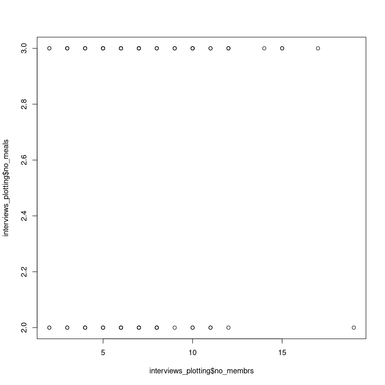
plot of chunk first-scatterplot
Scatterplots are useful for showing that sort for relationships in the data. Here it does not appear that the correlation exists; there is no clear trend.
We might want to adjust the labels on the axes, and add a main title:
plot(interviews_plotting$no_membrs, interviews_plotting$no_meals,
     main = "Relation between number of members of households, and number of meals served",
     xlab = "Years lived",
     ylab = "Items owned")
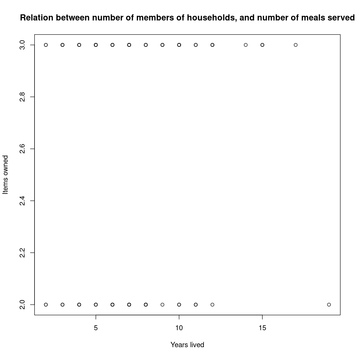
plot of chunk unnamed-chunk-2
Boxplots
We can use boxplots to visualize the distribution of number of household members for each wall type:
boxplot(interviews_plotting$no_membrs~interviews_plotting$respondent_wall_type)
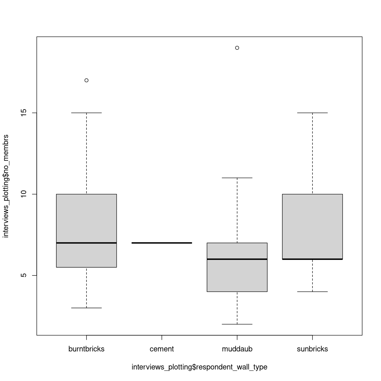
plot of chunk unnamed-chunk-3
Two new things happens here. First, we are using a new way of telling the plot function what relationship we want to visualise. The function notation y~x, tells the boxplot function that we want to visualise y as a function of x. In this case we want to visualise the number of people, as af function of the wall type. Secondly, we use a boxplot. A boxplots shows the distribution of the values on the y-axis. The median value is indicated by the solid bar. The box encapsulates 50% of the observations. Its upper and lower borders represents the interquartile range (IQR). The whiskers on the plot - here only the upper whiskers are shown due to the nature of the data, represents the range of the data. The distance from the upper part of the box, to the whisker is 1.5 times the interquartile range. The dots that we see for muddaub and sunbricks are outliers. Observations that lies so far from the rest of the observations, that we consider them as outliers.
Depending on the data, and the nature of the analyses we are going to do, outliers are either very interesting, or something that we can ignore.
Histograms
Another useful plottype are histograms.
hist(interviews_plotting$no_membrs)
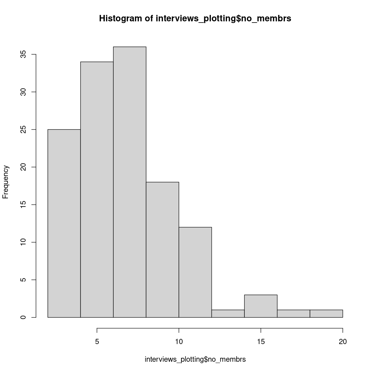
plot of chunk unnamed-chunk-4
Histograms counts the number of observations in our data, that lies between two values. Here the “breaks” between the values on the x-axis corresponds nicely to the number of people, but they do not have to.
Writing our own functions
When calculating an average of several values, we do two things. First we count how many values there are. Then we sum all the values, and divides the sum by the number of values. Rather than writing R-code for each of these three operations, we use the mean() function, where other more experienced programmers have written the code.
We can write our own functions, where we collect several operations into one function.
Functions in R are defined in this way:
function_name <- function(x){
  temporary_result_1 <- some_function(x)
  temporary_result_2 <- some_other_function(temporary_result_1)
  yet_another_function(temporary_result_2)
}
function_name defines the name of our function.
function(x) tells R that we are defining a function, that takes X as input. We can then use that x as input to calculations or other functions within our own function.
Between the curly braces {}, we define what we want our function to do. We assign the result of some_function(x) to a temporary result, use that as the input to a second function, and the result of that as the input to a third function. The result of the last calculation we do, will be returned as the output of our function.
Exercise
Write a function that calculates the average value of a numeric vector, takes the square root of that average, and returns the result
Solution
One way to do this would be:
root_mean <- function(x){ sqrt(mean(x, na.rm=T)) }
Another way could be:
root_mean <- function(x){ temp <- mean(x, na.rm =T) result <- sqrt(temp) result }
Logical tests in functions
Some times we want to do something different to the data, depending on the data. We can control the flow of the code using the if() construction.
As an example: if(x<10){ print(“X is smaller than 10”) }else{ print(“x is larger than 10”) }
The if() function will run the code provided in the curly braces {}, if, and
only if, the expression in the paranthesis is true. If x is 11, x is not
smaller than 10, and the first print function will not be executed.
The else-part is not requiered, but normally we will have to execute some other code if the statement in the if-function is not true. In this case if x is 11, the first print-function will not be executed, but the second will.
We use logical tests to handle data differently, depending on some characteristics of the data.
loops
Loops are constructs we use to do the same operations on lots of data.
for loops
For loops are constructs used to apply one or more functions on a series of data.
for(i in 1:10){
  temp <- sqrt(i)
  print(temp)
}
[1] 1
[1] 1.414214
[1] 1.732051
[1] 2
[1] 2.236068
[1] 2.44949
[1] 2.645751
[1] 2.828427
[1] 3
[1] 3.162278
will take every value in the vector 1:10, the digits 1 to 10, one by one, assign it to a temporary variable i and run the code we write in the curly braces. Here the for-loop will take all numbers from 1 to 10, calculate the squareroot of them. The result is assigned to another temporary variable “temp” and then temp is printed.
Danger Will Robinson
As a general rule, R does not handle loops very efficiently. This is a simple loop, operating on only 10 values, and we wont notice the difference in speed.
But we can measure it.
The Sys.time() function will tell us what time our computer thinks it is. If we run that just before, and just after our loop, we can calculate how long it took to run.
tic <- Sys.time()
for(i in 1:1000){
  temp <- sqrt(i)
  print(temp)
}
toc <- Sys.time()
for_time <- toc - tic
A more efficient way to calculate the square root of the numbers from 1 to 10 would be use the fact that sqrt() is a vectorized function that will calculate the square root of every element in a vector used as input to it:
tic <- Sys.time()
sqrt(1:1000)
toc <- Sys.time()
vect_time <- toc - tic
vect_time
And we can then compare how much faster the latter vectorized solution is.
as.numeric(for_time)/as.numeric(vect_time)
[1] 5.941002
More than double as fast! To be fair most of the time is spent outputting the results, but as a general rule utilizing the vectorized nature of functions is faster than writing loops. But that is not always a luxury we have.
while loops
While loops are loops that execute the code - as long as some criterium is satisfied.
i <- 1
while(i <= 10){
  print(sqrt(i))
  i <- i + 1
}
[1] 1
[1] 1.414214
[1] 1.732051
[1] 2
[1] 2.236068
[1] 2.44949
[1] 2.645751
[1] 2.828427
[1] 3
[1] 3.162278
This loop structure does the exact same as the two previous examples. Here we need to assign an initial value i, and then our while loop will execute the code within the curly braces, as long as i is smaller than or equal to 10. It is important to remember to increment the value of i - otherwise i will always be 1, and therefore always smaller than 10. And the loop will never stop.
ggplot
The plotting functions in R produce nice clean plots without any fancy details. That is generally a good thing, we want to maximize the information per ink in our plots.
However, we are limited in the types of plots we can make, and sometimes we just want a bit more color.
Enter ggplot2.
ggplot2 is a package designed to work well with the packages we have already encountered. It produces plots in a structured way, and comes with a lot of extensions, that enables us to plot almost anything.
The basic structure of ggplots are:
ggplot(data, mapping = aes(x=x, y=y)) +
  geom_point()
ggplot takes some data. Typically we will provide the data using the pipe: ` %>% `
data %>%
  ggplot(mapping = aes(x=x, y=y)) +
    geom_point()
The mapping argument tells ggplot which variables in our data should be mapped
to the x- and y-axes in our plot.
That in itself will not produce much of a plot. We need to tell ggplot which type of plot we want.
We do that by adding a geom_ function. Here we have added geom_point which
produces a scatter-plot. Other functions are more intuitively named. geom_col
gives us a column-plot, geom_histogram a histogram etc.
Let us try to make a histogram like we saw earlier:
interviews_plotting %>%
  ggplot(aes(x=no_membrs)) +
  geom_histogram()
`stat_bin()` using `bins = 30`. Pick better value with `binwidth`.
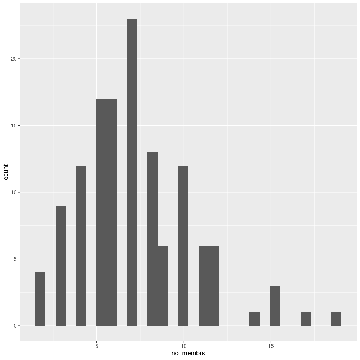
plot of chunk unnamed-chunk-14
It looks different, and we get a warning about binwidth. geom_histogram automatically
chooses 30 bins for us, and that is normally not the right number.
Key Points
Boxplots are useful for visualizing the distribution of a continuous variable.
Barplots are useful for visualizing categorical data.
Functions allows you to repeat the same set of operations again and again.
Loops allows you to apply the same function to lots of data.
Logical tests allow you to apply different calculations on different sets of data.
What is the next step?
Overview
Teaching: 10 min
Exercises: 0 minQuestions
What do I do now?
What is the next step?
Objectives
Present suggestions for further reading,
Tips on problems to work on to practice,
Great sites
What should I practice on?
Contact us!
The whole reason for the existence of KUB Datalab is to help and assist students (and teachers and researchers) working with data.
We do not guarantee that we will be able to solve your problems, but we will do our best to help you.
Our calender, containing our activities, courses, seminars, datasprints etc.
Our website
Our mail: kubdatalab@kb.dk
Key Points
Practice is important!
Working on data that YOU find interesting is a really good idea,
The amount of ressources online is immense.
KUB Datalab is there for your.