All in One View
Content from What is an API?
Last updated on 2026-07-07 | Edit this page
Estimated time: 12 minutes
Overview
Questions
- What is an API?
- How do our computer interact with servers?
Objectives
- Understand what an API do
- Get to know the two main ways to get data from APIs
What is an API?
An API is an Application Programming Interface. It is a way of making applications, in our case an R-script, able to communicate with another application typically an online database.
What we want to be able to do, is to let our own application, our R-script, send a command to a remote application, an online database, in order to retrieve specific data.
And we want to read the answer we get in return.
This is equivalent to requesting a page from a webserver, something we have all done.
Webservers and browsers communicate using the HTTP protocol, and the mechanics of this communication can be visualized like this:
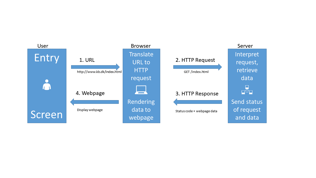
When we type in an URL in our browser, it translates that URL to a HTTP-request.
The browser sends that HTTP-request to a webserver. The request contains information about the page we need, but in the “header” of the request, there is a lot of other information. The version of browser we are using and cookies, to just mention two. The most important might be information about what type of response we would like.
The webserver interpret the request, and retrieves the data.
After that, the webserver sends both the status of the request (hopefully 200 - which is short for “everything is OK”), and the data.
The browser receives the data, and displays it as a webpage.
When we are working with APIs we cut out the user. We have a script that needs some data. We write code that defines, and then send a request til a server, specifying which data we need. The server extracts the needed data, and returns it to the script.
So - how do we do that?
Looking closer at the illustration above, we can see that we send a request to the server. That request contains several parts.
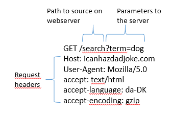
The request line. That contains the method we are using to communicate with the server, the address and path of the server, and the information about the version of HTTP we are using to communicate with the server.
The header. Headers are meta information about our request. It contains information about who we are, the type of browser we are using and much more.
The body. This is really the message that we are sending to the server. Where the request line tells our computer where to we are sending our request, and the header provides information about the request, the body is the actual message we are sending to the server.
The trick is now to make the API understand what data we would like to get back from it.
Two types of requests
Two main types of requests are used when communicating with APIs, and they primarily concerns how we tell the API what data we would like.
In a GET request, we encode what we would like returned in the URL. You probably know that way already.
The URL “https://icanhazdadjoke.com/search?term=dog” is asking the server to search for the term “dog”. What we are searching for, is placed directly in the URL.
What we are sending to the server looks like this:
In a POST request, that information is stored in the body of the request.
That looks like this:
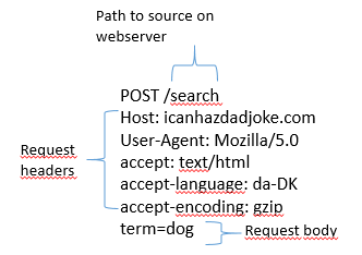
Note that the main difference between these two sets of headers, besides the difference in GET and POST, is that there is a body in the POST version. This is where the actual search is placed, rather than in the URL.
Almost all APIs support one or both of these methods.
The GET method is intuitively easy to understand, and it is relatively easy to edit the URL to search for something else. On the other hand there are limitations to what we can search for. Everything must be text, and there are limitations on the length of the search as well.
The POST method allow us to search for arbitrarily many parameters, and can handle many different data types - because we can put almost any kind of data into the body part of the request. The POST method is also more secure, because the body can be encrypted during transport from our computer to the server. This is also the method we need to use should the API require a login.
- Getting data from an API is equivalent to requesting a webpage
- GET requests specify what data we want to retrieve in the URL
- POST requests specify what data we want to retrieve in the body of the request.
- Both requests have headers that we can manipulate to get what we want.
Content from GETting data
Last updated on 2026-07-07 | Edit this page
Estimated time: 12 minutes
Overview
Questions
- How do I get data from an API using the GET method?
- Is there a way to modify headers, to get a specific type of result?
Objectives
- Learn how to retrieve data using the GET method
- Learn how to adjust headers to get desired result
Please note: These pages are autogenerated. Some of the API-calls may fail during that process. We are figuring out what to do about it, but please excuse us for any red errors on the pages for the time being.
Using GET
The site icanhazdadjoke.com offers a wide selection of dad-jokes.
Dad jokes
a wholesome joke of the type said to be told by fathers with a punchline that is often an obvious or predictable pun or play on words and usually judged to be endearingly corny or unfunny. According to Merriam Webster
In addition to the website, an API is available that can be accessed using the GET method.
The GET method is a generic procedure, we need a function that actually handles the behind-the-scenes-stuff for us. The library httr have an implementation:
R
library(httr)
Taking a quick look at the documentation we first try GET directly:
R
GET("https://icanhazdadjoke.com/")
OUTPUT
Response [https://icanhazdadjoke.com/]
  Date: 2026-07-07 01:51
  Status: 200
  Content-Type: text/html; charset=utf-8
  Size: 11.7 kB
<!DOCTYPE html>
<html lang="en">
  <head>
    <meta charset="utf-8">
    <meta http-equiv="X-UA-Compatible" content="IE=edge">
    <meta name="viewport" content="width=device-width, initial-scale=1, minim...
    <meta name="description" content="The largest collection of dad jokes on ...
    <meta name="author" content="C653 Labs" />
    <meta name="keywords" content="dad,joke,funny,slack,alexa" />
    <meta property="og:site_name" content="icanhazdadjoke" />
...
What is returned is the response from the server. That includes much more than what we are looking for. Notable is the “Status” part, which we are told is “200”, which is server-lingo for “everything is OK”.
And what do we get? We get a webpage. We can see that the content is DOCTYPE html. That was not really what we were looking for. HTML is not that easy to work with, and contains a lot of extranious information that we do not need.
Even if the GET method is relatively simple to work with, we need to add a bit more. Again taking a look at the documentation, it appears that we need to tell the API, that we would like a specific type of response, rather than the default html, more specifically “text/plain”.
httr has helper functions to assist us. The one we need
here is accept() We now use that to tell the server, that
we really want a response in just text:
R
result <- GET("https://icanhazdadjoke.com/", accept("text/plain"))
result
OUTPUT
Response [https://icanhazdadjoke.com/]
  Date: 2026-07-07 01:51
  Status: 200
  Content-Type: text/plain
  Size: 102 B
We still get the response from the server, telling us that Status is 200, and everything is OK. But where is our dad-joke?
It is hidden in the content of the response. It is sent to us as
binary code, so we are using the content() function, also
from httr to extract it:
R
content(result)
OUTPUT
No encoding supplied: defaulting to UTF-8.OUTPUT
[1] "Dad died because he couldn't remember his blood type. I will never forget his last words. Be positive."There is a little warning about the encoding of the string. But now we have a dad-joke!
What if we need to retrieve a specific joke? All the jokes has an ID, that we can use for that. If we want to find that, we need a bit more information about the joke. We can get that by specifying that we would like the result of our GET-request returned as JSON.
JSON
JSON (JavaScript Object Notation) is a format for structuring, in principle, any kind for text, structured in almost any way. It consists of pairs of strings, one denoting the name of the data we are looking at, and one containing the content of that data. Each set of data fields are encapsulated in curly braces, and a data field can have subfields, also encapsulated in curly braces. It can look like this:
{ “firstName”: “John”, “lastName”: “Smith”, “phoneNumbers”:{ “type”: “home”, “number”: “212 555-1234” }, { “type”: “office”, “number”: “646 555-4567” } }
Which translates to a table like this:
| firstName | lastName | phoneNumbers | ||||||
|---|---|---|---|---|---|---|---|---|
| John | Smith |
|
JSON is readable for both humans and computers, but can be a bit tricky to convert to dataframes if there are a lot of nested fields.
Looking at the documentation, we see an example, which indicates that
what we should tell the server that we accept, should be
“application/json”. The httr library contains helper
functions to assist us in manipulating the header. We use
accept() that sets the accept part of the
header:
R
result <- GET("https://icanhazdadjoke.com/", accept("application/json"))
result
OUTPUT
Response [https://icanhazdadjoke.com/]
  Date: 2026-07-07 01:51
  Status: 200
  Content-Type: application/json
  Size: 89 B
{"id":"cUnWLRZ01wc","joke":"What is the leading cause of dry skin? Towels","s...
Again - everything is nice and 200 = OK.
We also see a truncated version of the actual joke.
Let us use the content() function to extract the
content:
R
content(result)
OUTPUT
$id
[1] "cUnWLRZ01wc"

$joke
[1] "What is the leading cause of dry skin? Towels"

$status
[1] 200
This data is returned as a list, which is the R-default way of handling any kind of data. Status is repeated, and now we have an id. We can use that to extract the same joke again.
NOTE: The joke returned is chosen at random. The id used here will probably be different from what we found above.
The way to retrieve a specific joke is to GET the URL:
GET https://icanhazdadjoke.com/j/<joke_id>
Where we replace the joke_id with the specific joke we want. Remember to specify the result that we want:
R
library(tidyverse)
GET("https://icanhazdadjoke.com/j/lGJmrrzAsc",  accept("text/plain")) |>
  content()
OUTPUT
No encoding supplied: defaulting to UTF-8.OUTPUT
[1] "A termite walks into a bar and asks “Is the bar tender here?”"We can also search for words in jokes. The documentation tells us, that we should send our GET request to the URL
https://icanhazdadjoke.com/search
And in the examples we get the hint, that we should format the URL as:
https://icanhazdadjoke.com/search?term=
Dogs are always fun, let us search for dad jokes about dogs. Specify
the type of result we want, pipe the response to the
content() function and save it to result (the
length has been edited):
R
result <- GET("https://icanhazdadjoke.com/search?term=dog",
              accept("application/json")) |>
          content()
result
OUTPUT
$current_page
[1] 1

$limit
[1] 20

$next_page
[1] 1

$previous_page
[1] 1

$results
$results[[1]]
$results[[1]]$id
[1] "YvkV8xXnjyd"

$results[[1]]$joke
[1] "Why did the cowboy have a weiner dog? Somebody told him to get a long little doggy."


$results[[2]]
$results[[2]]$id
[1] "82wHlbaapzd"

$results[[2]]$joke
[1] "Me: If humans lose the ability to hear high frequency volumes as they get older, can my 4 week old son hear a dog whistle?\r\n\r\nDoctor: No, humans can never hear that high of a frequency no matter what age they are.\r\n\r\nMe: Trick question... dogs can't whistle."


$results[[3]]
$results[[3]]$id
[1] "EBQfiyXD5ob"

$results[[3]]$joke
[1] "what do you call a dog that can do magic tricks? a labracadabrador"


$search_term
[1] "dog"

$status
[1] 200

$total_jokes
[1] 13

$total_pages
[1] 1
This is in JSON format. It is clear that the jokes are in the $results part of that datastructure. How can we get that to a data frame?
The content() function can treat the content of our
response in different ways. If we treat it as text, the function
fromJSON from the library jsonlite, can convert it to a
data frame. We begin by loading the library:
R
library(jsonlite)
GET("https://icanhazdadjoke.com/search?term=dog", accept("application/json")) |>
  content(as="text") |>
  fromJSON()
OUTPUT
$current_page
[1] 1

$limit
[1] 20

$next_page
[1] 1

$previous_page
[1] 1

$results
            id
1  YvkV8xXnjyd
2  82wHlbaapzd
3  EBQfiyXD5ob
4  GtH6E6UD5Ed
5   obhFBljb2g
6  89MZLmWnWvc
7   71wsPKeF6h
8  R7UfaahVfFd
9  lyk3EIBQfxc
10 DIeaUDlbUDd
11 AQn3wPKeqrc
12 sPRnOfiyAAd
13 Lmjqzsr49pb
                                                                                                                                                                                                                                                                         joke
1                                                                                                                                                                                         Why did the cowboy have a weiner dog? Somebody told him to get a long little doggy.
2  Me: If humans lose the ability to hear high frequency volumes as they get older, can my 4 week old son hear a dog whistle?\r\n\r\nDoctor: No, humans can never hear that high of a frequency no matter what age they are.\r\n\r\nMe: Trick question... dogs can't whistle.
3                                                                                                                                                                                                          what do you call a dog that can do magic tricks? a labracadabrador
4                                                                                                                                                                                                What kind of dog lives in a particle accelerator? A Fermilabrador Retriever.
5                                                                                                                                                                                     I adopted my dog from a blacksmith. As soon as we got home he made a bolt for the door.
6                                                                                                                                                I can't take my dog to the pond anymore because the ducks keep attacking him. That's what I get for buying a pure bread dog.
7                                                                                                                                                                                                                           What did the dog say to the two trees? Bark bark.
8                                                                                                                                                                                     My dog used to chase people on a bike a lot. It got so bad I had to take his bike away.
9                                                                                                                                                                                             I went to the zoo the other day, there was only one dog in it. It was a shitzu.
10                                                                                                                                                                                                                         “My Dog has no nose.” “How does he smell?” “Awful”
11                                                                                                                                                                                                  It was raining cats and dogs the other day. I almost stepped in a poodle.
12                                                                                                                                              At the boxing match, the dad got into the popcorn line and the line for hot dogs, but he wanted to stay out of the punchline.
13                                                                                                                                                                                            What did the Zen Buddist say to the hotdog vendor? Make me one with everything.

$search_term
[1] "dog"

$status
[1] 200

$total_jokes
[1] 13

$total_pages
[1] 1
We have now seen how to send a request to an API, with search terms embedded in the URL.
We have seen how to add an argument to the GET function, that specifies the type of result we would like, effectively by adding something to the header of our request.
And we have seen how to extract the results, and get them into a dataframe.
Next, we are going to take a look on how we get results using the POST method, on an API that provides more factual and serious, but not so funny data.
Exercise
Request dad jokes about cats using the GET() function,
and extract the content.
We’ve done this earlier, and just have to change “dog” to “cat”:
R
GET("https://icanhazdadjoke.com/search?term=cat", accept("application/json")) |>
content(as="text") |>
fromJSON()
OUTPUT
No encoding supplied: defaulting to UTF-8.OUTPUT
$current_page
[1] 1

$limit
[1] 20

$next_page
[1] 1

$previous_page
[1] 1

$results
            id
1  iGJeVKmWDlb
2   8UnrHe2T0g
3     daaUfibh
4  TS0gFlqr4ob
5  O7haxA5Tfxc
6  0wcFBQfiGBd
7  0DdaxAX0orc
8    39Etc2orc
9  BQfaxsHBsrc
10 1wkqrcNCljb
11 AQn3wPKeqrc
                                                                                  joke
1                  My cat was just sick on the carpet, I don’t think it’s feline well.
2                                 ‘Put the cat out’ … ‘I didn’t realize it was on fire
3            Why was the big cat disqualified from the race? Because it was a cheetah.
4                      What do you call a group of disorganized cats? A cat-tastrophe.
5                                         Where do cats write notes?\r\nScratch Paper!
6             Did you hear the joke about the wandering nun? She was a roman catholic.
7                         I accidentally took my cats meds last night. Don’t ask meow.
8  Why did the man run around his bed? Because he was trying to catch up on his sleep!
9                                        What do you call a pile of cats?  A Meowtain.
10         Did you know that protons have mass? I didn't even know they were catholic.
11           It was raining cats and dogs the other day. I almost stepped in a poodle.

$search_term
[1] "cat"

$status
[1] 200

$total_jokes
[1] 11

$total_pages
[1] 1- 200 is the internet code for everything is OK
- GET requests can be adjusted to specify desired result
- Dad jokes are not really that funny.
Content from Using POST
Last updated on 2026-07-07 | Edit this page
Estimated time: 45 minutes
Overview
Questions
- How do I get data from an API using the POST method?
Objectives
- Connect to Statistics Denmark, and extract data
- Create a list of lists to control the variables to be extracted
Please note: These pages are autogenerated. Some of the API-calls may fail during that process. We are figuring out what to do about it, but please excuse us for any red errors on the pages for the time being.
Getting data from Statistics Denmark
The API from statistics Denmark can accept GET requests. But they recommend using POST instead. That allows us to do more advanced searches for data easier.
We are going to write a POST-request (with a little help from R), to retrieve data from Statistics Denmark.
But before we can do that, we need to know how the Statistics Denmark API expects to receive data.
Hopefully we can get that by reading the documentation, that can be found here.
But that is rather confusing.
The main points:
First: Statistics Denmark provides four “functions”, or endpoints. This is equivalent to the URL we requested data from using the GET method.
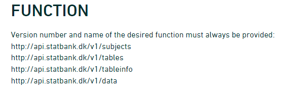
- The first is the “web”-site we have to send requests to if we want information on the subjects in Statistics Denmark.
- In the second we get information about which tables are available for a given subject.
- The third will provide metadata on a table.
- When we finally need the data, we will visit the last endpoint.
Secondly: We need to provide a body containing search parameters in a format like this:
R
{
   "table": "folk1c"
}
Let us look at how to do this, by sending a request to
subjects.
The endpoint was
R
endpoint <- "http://api.statbank.dk/v1/subjects"
We will now need to construct a named list for the content of the body that we send along with our request.
This is a new datastructure that we have not encountered before.
Vectors are annoying because they can only contain one datatype. And dataframes must be rectangular.
A list allows us to store basically anything. The reason that we do not use them for everything is that they are a bit more difficult to work with.
R
our_body <- list(lang = "en", recursive = FALSE,
                  includeTables = FALSE, subjects = NULL)
This list contains four elements, with names. - The first,
lang, contains a character vector (length 1), containing
“en”, the language that we want Statistics Denmark to use when returning
data. - recursive and includeTables are
logical values, both false. - subjects is a special value,
NULL. This is not a missing value, there simply isn’t anything there.
But this nothing does have a name.
lists
Lists are subset in a special way. If we want the first element in
our_body, we can use the usual bracket notation:
R
our_body[1]
OUTPUT
$lang
[1] "en"
If we want the actual value of element 1, we use a double bracket notation:
R
our_body[[1]]
OUTPUT
[1] "en"Now we have the two things we need, an endpoint to send a request, and a body containing what we want returned.
Let us try it:
R
result <- httr::POST(endpoint, body=our_body, encode = "json")
We specify that the request should be encoded as “json”.
Let us look at the result:
R
result
OUTPUT
Response [https://api.statbank.dk/v1/subjects]
  Date: 2026-07-07 01:51
  Status: 200
  Content-Type: text/json; charset=utf-8
  Size: 903 B
Both informative. And utterly useless. The informative information is that our request succeeded (cave - it might not succeed on this webpage). We can see that in the status. 200 is an internet code for success.
Let us get the content of the result, which is what we actually want:
R
result |>
  content()
OUTPUT
[1] "[{\"id\":\"1\",\"description\":\"People\",\"active\":true,\"hasSubjects\":true,\"subjects\":[]},{\"id\":\"2\",\"description\":\"Labour and income\",\"active\":true,\"hasSubjects\":true,\"subjects\":[]},{\"id\":\"3\",\"description\":\"Economy\",\"active\":true,\"hasSubjects\":true,\"subjects\":[]},{\"id\":\"4\",\"description\":\"Social conditions\",\"active\":true,\"hasSubjects\":true,\"subjects\":[]},{\"id\":\"5\",\"description\":\"Education and research\",\"active\":true,\"hasSubjects\":true,\"subjects\":[]},{\"id\":\"6\",\"description\":\"Business\",\"active\":true,\"hasSubjects\":true,\"subjects\":[]},{\"id\":\"7\",\"description\":\"Transport\",\"active\":true,\"hasSubjects\":true,\"subjects\":[]},{\"id\":\"8\",\"description\":\"Culture and leisure\",\"active\":true,\"hasSubjects\":true,\"subjects\":[]},{\"id\":\"9\",\"description\":\"Environment and energy\",\"active\":true,\"hasSubjects\":true,\"subjects\":[]},{\"id\":\"19\",\"description\":\"About Statistics Denmark\",\"active\":true,\"hasSubjects\":true,\"subjects\":[]}]"More informative, but not really easy to read.
The library jsonlite has a function that converts this
to something readable:
R
result |>
  content() |>
  fromJSON()
OUTPUT
   id              description active hasSubjects subjects
1   1                   People   TRUE        TRUE     NULL
2   2        Labour and income   TRUE        TRUE     NULL
3   3                  Economy   TRUE        TRUE     NULL
4   4        Social conditions   TRUE        TRUE     NULL
5   5   Education and research   TRUE        TRUE     NULL
6   6                 Business   TRUE        TRUE     NULL
7   7                Transport   TRUE        TRUE     NULL
8   8      Culture and leisure   TRUE        TRUE     NULL
9   9   Environment and energy   TRUE        TRUE     NULL
10 19 About Statistics Denmark   TRUE        TRUE     NULL
A nice dataframe with the ten major subjects in the databases of Statistics Denmark.
Subject 1 contains information about populations and elections.
There are sub-subjects under that. We can see that in the column
hasSubjects
We now modify our body that we send with the request, to return information about the first subject.
We need to make sure that the number of the subject, 1
is intepreted as it is. This is a little bit of mysterious handwaving -
we simply put the 1 inside the function I() and stuff
works.
R
our_body <- list(lang = "en", recursive = F,
                  includeTables = F, subjects = I(1))
I()
I() isolates - or insulates - the contents of
I() from the gaze of R’s parsing code. Basically it
prevents R from doing stuff to the content that we dont want it to. In
this specific case, the POST() function would convert the
vector 1, with length 1, to a scalar, the more basic data type in R,
that hold only one, single, atomic value at a time.
Note that it is important that we tell the POST()
function that the body is the body:
R
data <- POST(endpoint, body=our_body, encode = "json") |>
  content() |>
  fromJSON()

data
OUTPUT
  id description active hasSubjects
1  1      People   TRUE        TRUE
                                                                                                                                                                                                                                                   subjects
1 3401, 3407, 3410, 3415, 3412, 3411, 3428, 3409, Population, Households and family matters , Migration, Housing, Health, Democracy, National church, Names, TRUE, TRUE, TRUE, TRUE, TRUE, TRUE, TRUE, TRUE, TRUE, TRUE, TRUE, TRUE, TRUE, TRUE, TRUE, TRUE
Not that easy to see in this format, but the data frame contains a
data frame. That is, in the column subjects the content is
a data frame.
We pick that out using the $-notation:
R
data$subjects
OUTPUT
[[1]]
    id                    description active hasSubjects subjects
1 3401                     Population   TRUE        TRUE     NULL
2 3407 Households and family matters    TRUE        TRUE     NULL
3 3410                      Migration   TRUE        TRUE     NULL
4 3415                        Housing   TRUE        TRUE     NULL
5 3412                         Health   TRUE        TRUE     NULL
6 3411                      Democracy   TRUE        TRUE     NULL
7 3428                National church   TRUE        TRUE     NULL
8 3409                          Names   TRUE        TRUE     NULL
These are the sub-subjects of subject 1.
Let us look closer at 3401, Population.
Again, we modify the call we send to the endpoint:
R
our_body <- list(lang = "en", recursive = F,
                  includeTables = F, subjects = I(3401))
R
data <- POST(endpoint, body=our_body, encode = "json") |>
  content() |>
  fromJSON()

data
OUTPUT
    id description active hasSubjects
1 3401  Population   TRUE        TRUE
                                                                                                                                                                                                                                                                                              subjects
1 20021, 20024, 20022, 20019, 20017, 20018, 20014, 20015, Population figures, Immigrants and their descendants, Population projections, Adoptions, Births, Fertility, Deaths, Life expectancy, TRUE, TRUE, TRUE, FALSE, TRUE, TRUE, TRUE, TRUE, FALSE, FALSE, FALSE, FALSE, FALSE, FALSE, FALSE, FALSE
We delve deeper into it:
R
data$subjects
OUTPUT
[[1]]
     id                      description active hasSubjects subjects
1 20021               Population figures   TRUE       FALSE     NULL
2 20024 Immigrants and their descendants   TRUE       FALSE     NULL
3 20022           Population projections   TRUE       FALSE     NULL
4 20019                        Adoptions  FALSE       FALSE     NULL
5 20017                           Births   TRUE       FALSE     NULL
6 20018                        Fertility   TRUE       FALSE     NULL
7 20014                           Deaths   TRUE       FALSE     NULL
8 20015                  Life expectancy   TRUE       FALSE     NULL
And now we are at the bottom. 20021 Population figures does not have any sub-sub-subjects.
Next, let us take a look at the tables contained under subject 20021.
We need the next endpoint, which provides information about tables under a subject:
R
endpoint <- "http://api.statbank.dk/v1/tables"
R
our_body <- list(lang = "en", subjects = I(20021))
data <- POST(endpoint, body=our_body, encode = "json") |>
  content() |>
  fromJSON()
data |> head()
OUTPUT
       id                                       text   unit             updated
1  FOLK1A Population at the first day of the quarter Number 2026-05-11T08:00:00
2 FOLK1AM   Population at the first day of the month Number 2026-06-10T08:00:00
3 BEFOLK3                      Population 1. January Number 2026-07-01T08:00:00
4 BEFOLK1                      Population 1. January Number 2026-02-12T08:00:00
5 BEFOLK2                      Population 1. January Number 2026-02-12T08:00:00
6   FOLK3                      Population 1. January Number 2026-02-12T08:00:00
  firstPeriod latestPeriod active
1      2008Q1       2026Q2   TRUE
2     2021M10      2026M05   TRUE
3        2008         2026   TRUE
4        1971         2026   TRUE
5        1901         2026   TRUE
6        2008         2026   TRUE
                                       variables
1         region, sex, age, marital status, time
2                         region, sex, age, time
3                         region, sex, age, time
4                 sex, age, marital status, time
5                                 sex, age, time
6 day of birth, birth month, year of birth, time
There are 21 tables under this subject. Let us see what information we can get about table “FOLK1A”:
We now need the third endpoint:
R
endpoint <- "http://api.statbank.dk/v1/tableinfo"
R
our_body <- list(lang = "en", table = "FOLK1A")
data <- POST(endpoint, body=our_body, encode = "json") |>
  content() |>
  fromJSON()
data
OUTPUT
$id
[1] "FOLK1A"
$text
[1] "Population at the first day of the quarter"
$description
[1] "Population at the first day of the quarter by region, sex, age, marital status and time"
$unit
[1] "Number"
$suppressedDataValue
[1] "0"
$updated
[1] "2026-05-11T08:00:00"
$active
[1] TRUE
$contacts
name phone mail
1 Dorthe Larsen +4523498326 dla@dst.dk
$documentation
$documentation$id
[1] "4a12721d-a8b0-4bde-82d7-1d1c6f319de3"
$documentation$url
[1] "https://www.dst.dk/documentationofstatistics/4a12721d-a8b0-4bde-82d7-1d1c6f319de3"
$footnote
NULL
$variables
id text elimination time map
1 OMRÅDE region TRUE FALSE denmark_municipality_07
2 KØN sex TRUE FALSE <NA>
3 ALDER age TRUE FALSE <NA>
4 CIVILSTAND marital status TRUE FALSE <NA>
5 Tid time FALSE TRUE <NA>
values
1 000, 084, 101, 147, 155, 185, 165, 151, 153, 157, 159, 161, 163, 167, 169, 183, 173, 175, 187, 201, 240, 210, 250, 190, 270, 260, 217, 219, 223, 230, 400, 411, 085, 253, 259, 350, 265, 269, 320, 376, 316, 326, 360, 370, 306, 329, 330, 340, 336, 390, 083, 420, 430, 440, 482, 410, 480, 450, 461, 479, 492, 530, 561, 563, 607, 510, 621, 540, 550, 573, 575, 630, 580, 082, 710, 766, 615, 707, 727, 730, 741, 740, 746, 706, 751, 657, 661, 756, 665, 760, 779, 671, 791, 081, 810, 813, 860, 849, 825, 846, 773, 840, 787, 820, 851, All Denmark, Region Hovedstaden, Copenhagen, Frederiksberg, Dragør, Tårnby, Albertslund, Ballerup, Brøndby, Gentofte, Gladsaxe, Glostrup, Herlev, Hvidovre, Høje-Taastrup, Ishøj, Lyngby-Taarbæk, Rødovre, Vallensbæk, Allerød, Egedal, Fredensborg, Frederikssund, Furesø, Gribskov, Halsnæs, Helsingør, Hillerød, Hørsholm, Rudersdal, Bornholm, Christiansø, Region Sjælland, Greve, Køge, Lejre, Roskilde, Solrød, Faxe, Guldborgsund, Holbæk, Kalundborg, Lolland, Næstved, Odsherred, Ringsted, Slagelse, Sorø, Stevns, Vordingborg, Region Syddanmark, Assens, Faaborg-Midtfyn, Kerteminde, Langeland, Middelfart, Nordfyns, Nyborg, Odense, Svendborg, Ærø, Billund, Esbjerg, Fanø, Fredericia, Haderslev, Kolding, Sønderborg, Tønder, Varde, Vejen, Vejle, Aabenraa, Region Midtjylland, Favrskov, Hedensted, Horsens, Norddjurs, Odder, Randers, Samsø, Silkeborg, Skanderborg, Syddjurs, Aarhus, Herning, Holstebro, Ikast-Brande, Lemvig, Ringkøbing-Skjern, Skive, Struer, Viborg, Region Nordjylland, Brønderslev, Frederikshavn, Hjørring, Jammerbugt, Læsø, Mariagerfjord, Morsø, Rebild, Thisted, Vesthimmerlands, Aalborg
2 TOT, 1, 2, Total, Men, Women
3 IALT, 0, 1, 2, 3, 4, 5, 6, 7, 8, 9, 10, 11, 12, 13, 14, 15, 16, 17, 18, 19, 20, 21, 22, 23, 24, 25, 26, 27, 28, 29, 30, 31, 32, 33, 34, 35, 36, 37, 38, 39, 40, 41, 42, 43, 44, 45, 46, 47, 48, 49, 50, 51, 52, 53, 54, 55, 56, 57, 58, 59, 60, 61, 62, 63, 64, 65, 66, 67, 68, 69, 70, 71, 72, 73, 74, 75, 76, 77, 78, 79, 80, 81, 82, 83, 84, 85, 86, 87, 88, 89, 90, 91, 92, 93, 94, 95, 96, 97, 98, 99, 100, 101, 102, 103, 104, 105, 106, 107, 108, 109, 110, 111, 112, 113, 114, 115, 116, 117, 118, 119, 120, 121, 122, 123, 124, 125, Age, total, 0 years, 1 year, 2 years, 3 years, 4 years, 5 years, 6 years, 7 years, 8 years, 9 years, 10 years, 11 years, 12 years, 13 years, 14 years, 15 years, 16 years, 17 years, 18 years, 19 years, 20 years, 21 years, 22 years, 23 years, 24 years, 25 years, 26 years, 27 years, 28 years, 29 years, 30 years, 31 years, 32 years, 33 years, 34 years, 35 years, 36 years, 37 years, 38 years, 39 years, 40 years, 41 years, 42 years, 43 years, 44 years, 45 years, 46 years, 47 years, 48 years, 49 years, 50 years, 51 years, 52 years, 53 years, 54 years, 55 years, 56 years, 57 years, 58 years, 59 years, 60 years, 61 years, 62 years, 63 years, 64 years, 65 years, 66 years, 67 years, 68 years, 69 years, 70 years, 71 years, 72 years, 73 years, 74 years, 75 years, 76 years, 77 years, 78 years, 79 years, 80 years, 81 years, 82 years, 83 years, 84 years, 85 years, 86 years, 87 years, 88 years, 89 years, 90 years, 91 years, 92 years, 93 years, 94 years, 95 years, 96 years, 97 years, 98 years, 99 years, 100 years, 101 years, 102 years, 103 years, 104 years, 105 years, 106 years, 107 years, 108 years, 109 years, 110 years, 111 years, 112 years, 113 years, 114 years, 115 years, 116 years, 117 years, 118 years, 119 years, 120 years, 121 years, 122 years, 123 years, 124 years, 125 years
4 TOT, U, G, E, F, Total, Never married, Married/separated, Widowed, Divorced
5 2008K1, 2008K2, 2008K3, 2008K4, 2009K1, 2009K2, 2009K3, 2009K4, 2010K1, 2010K2, 2010K3, 2010K4, 2011K1, 2011K2, 2011K3, 2011K4, 2012K1, 2012K2, 2012K3, 2012K4, 2013K1, 2013K2, 2013K3, 2013K4, 2014K1, 2014K2, 2014K3, 2014K4, 2015K1, 2015K2, 2015K3, 2015K4, 2016K1, 2016K2, 2016K3, 2016K4, 2017K1, 2017K2, 2017K3, 2017K4, 2018K1, 2018K2, 2018K3, 2018K4, 2019K1, 2019K2, 2019K3, 2019K4, 2020K1, 2020K2, 2020K3, 2020K4, 2021K1, 2021K2, 2021K3, 2021K4, 2022K1, 2022K2, 2022K3, 2022K4, 2023K1, 2023K2, 2023K3, 2023K4, 2024K1, 2024K2, 2024K3, 2024K4, 2025K1, 2025K2, 2025K3, 2025K4, 2026K1, 2026K2, 2008Q1, 2008Q2, 2008Q3, 2008Q4, 2009Q1, 2009Q2, 2009Q3, 2009Q4, 2010Q1, 2010Q2, 2010Q3, 2010Q4, 2011Q1, 2011Q2, 2011Q3, 2011Q4, 2012Q1, 2012Q2, 2012Q3, 2012Q4, 2013Q1, 2013Q2, 2013Q3, 2013Q4, 2014Q1, 2014Q2, 2014Q3, 2014Q4, 2015Q1, 2015Q2, 2015Q3, 2015Q4, 2016Q1, 2016Q2, 2016Q3, 2016Q4, 2017Q1, 2017Q2, 2017Q3, 2017Q4, 2018Q1, 2018Q2, 2018Q3, 2018Q4, 2019Q1, 2019Q2, 2019Q3, 2019Q4, 2020Q1, 2020Q2, 2020Q3, 2020Q4, 2021Q1, 2021Q2, 2021Q3, 2021Q4, 2022Q1, 2022Q2, 2022Q3, 2022Q4, 2023Q1, 2023Q2, 2023Q3, 2023Q4, 2024Q1, 2024Q2, 2024Q3, 2024Q4, 2025Q1, 2025Q2, 2025Q3, 2025Q4, 2026Q1, 2026Q2This is a bit more complicated. We are told that:
- there are five columns in this table.
- They each have an id
- And a descriptive text
- Elimination means that the API will attempt to eliminate the variables we have not chosen alues for when data is returned. This makes sense when we get to point 7.
- time - only one of the variables contain information about a point in time.
- One of the variables can be mapped to - well a map
- The final column provides information about which values are stored in the variable. There are 105 different regions in Denmark. And if we do not choose a specific region - the API will attempt to eliminate this facetting, and return data for all of Denmark.
These data provides useful information for constructing the final call to the API in order to get the data.
We will now need the final endpoint:
R
endpoint <- "http://api.statbank.dk/v1/data"
And we will need to specify which information, from which table, we want data in the body of the request. That is a bit more complicated. We need to make a list of lists!
We start by placing the individual lists within a list, and save that
to an object - variables:
R
variables <- list(list(code = "OMRÅDE", values = I("*")),
                  list(code = "CIVILSTAND", values = I(c("U", "G", "E", "F"))),
                  list(code = "Tid", values = I("*"))
              )
We can then embed that list into a new list, containing the entire body:
R
our_body <- list(table = "FOLK1A", lang = "en", format = "CSV", variables = variables)
The final call boils down to:
R
data <- POST(endpoint, body=our_body, encode = "json")
The data is returned as csv - we defined that in “our_body”, so we now need to extract it a bit differently:
R
data <- data |>
  content(type = "text") |>
  read_csv2()
WARNING
Warning: The `file` argument of `read_csv2()` should use `I()` for literal data as of
readr 2.2.0.

  # Bad (for example):
  read_csv("x,y\n1,2")

  # Good:
  read_csv(I("x,y\n1,2"))
This warning is displayed once per session.
Call `lifecycle::last_lifecycle_warnings()` to see where this warning was
generated.
R
data
OUTPUT
# A tibble: 31,080 × 4
   OMRÅDE      CIVILSTAND    TID    INDHOLD
   <chr>       <chr>         <chr>    <dbl>
 1 All Denmark Never married 2008Q1 2552700
 2 All Denmark Never married 2008Q2 2563134
 3 All Denmark Never married 2008Q3 2564705
 4 All Denmark Never married 2008Q4 2568255
 5 All Denmark Never married 2009Q1 2575185
 6 All Denmark Never married 2009Q2 2584993
 7 All Denmark Never married 2009Q3 2584560
 8 All Denmark Never married 2009Q4 2588198
 9 All Denmark Never married 2010Q1 2593172
10 All Denmark Never married 2010Q2 2604129
# ℹ 31,070 more rows
Voila! We have a dataframe with information about how many persons in Denmark were married (or not) at different points in time.
That was a bit complicated. There are easier ways to do it.
We will look at that shortly. So why do it this way? These techniques are the same techniques we use when we access an arbitrary other API. The fields, endpoints etc might be different. We might have an added complication of having to login to it. But the techniques can be reused.
If we want, we can save the data:
R
write_csv2(data, "/data/SD_data.csv")
Remember to make a data folder before trying to save
data in it.
- POST requests to servers put specific demands on how we request data
- Using an API requires us to understand (some of) the ways the API works
- Different searches typically requires different endpoints
Content from What about danstat?
Last updated on 2026-07-07 | Edit this page
Estimated time: 12 minutes
Overview
Questions
- Is there an easier way to access Statistics Denmark?
Objectives
- Use a package to do the API-calls to Statistics Denmark
- Connect to Statistics Denmark, and extract data
- Create a list of lists to control the variables to be extracted
- Using the danstat package
Please note: These pages are autogenerated. Some of the API-calls may fail during that process. We are figuring out what to do about it, but please excuse us for any red errors on the pages for the time being.
Is there an easier way?
Many larger online services provide packages for easier access to their APIs.
Popular services might not have to do this, because enthusiasts write packages themselves.
A package called danstat is available, and makes it
easier to extract data from Statistics Denmark.
The danstat package/library
Previously we retrieved at table with demographic data from Statistics Denmark.
How can we get that table using the danstat package?
Before using the library, we will need to install it:
R
install.packages("danstat")
Some installations of R may have problems installing it. In that case, try this:
R
install.packages("remotes")
library(remotes)
remotes:install_github("cran/danstat")
After installation, we load the library using the library function. And then we can access the functions included in the library:
The danstat package contain four functions, equivalent to the four endpoints we discussed earlier.
The get_subjects() function sends a request to the
Statistics Denmark API, asking for a list of the subjects. The
information is returned to our script, and the
get_subjects() function presents us with a dataframe
containing the information.
R
library(danstat)
subjects <- get_subjects()
subjects
OUTPUT
   id              description active hasSubjects subjects
1   1                   People   TRUE        TRUE     NULL
2   2        Labour and income   TRUE        TRUE     NULL
3   3                  Economy   TRUE        TRUE     NULL
4   4        Social conditions   TRUE        TRUE     NULL
5   5   Education and research   TRUE        TRUE     NULL
6   6                 Business   TRUE        TRUE     NULL
7   7                Transport   TRUE        TRUE     NULL
8   8      Culture and leisure   TRUE        TRUE     NULL
9   9   Environment and energy   TRUE        TRUE     NULL
10 19 About Statistics Denmark   TRUE        TRUE     NULL
We get the 10 major subjects from Statistics Denmark we have seen before. As before, each of them have sub-subjects.
If we want to take a closer look at the subdivisions of a given
subject, we use the get_subjects() function again, this
time specifying which subject we are interested in:
Let us try to get the sub-subjects from the subject 1 - containing information about populations and elections:
R
sub_subjects <- get_subjects(subjects = 1)
sub_subjects
OUTPUT
  id description active hasSubjects
1  1      People   TRUE        TRUE
                                                                                                                                                                                                                                                   subjects
1 3401, 3407, 3410, 3415, 3412, 3411, 3428, 3409, Population, Households and family matters , Migration, Housing, Health, Democracy, National church, Names, TRUE, TRUE, TRUE, TRUE, TRUE, TRUE, TRUE, TRUE, TRUE, TRUE, TRUE, TRUE, TRUE, TRUE, TRUE, TRUE
The result is a bit complicated. The column “subjects” in the resulting dataframe contains another dataframe. We access it like we normally would access a column in a dataframe:
R
sub_subjects$subjects
OUTPUT
[[1]]
    id                    description active hasSubjects subjects
1 3401                     Population   TRUE        TRUE     NULL
2 3407 Households and family matters    TRUE        TRUE     NULL
3 3410                      Migration   TRUE        TRUE     NULL
4 3415                        Housing   TRUE        TRUE     NULL
5 3412                         Health   TRUE        TRUE     NULL
6 3411                      Democracy   TRUE        TRUE     NULL
7 3428                National church   TRUE        TRUE     NULL
8 3409                          Names   TRUE        TRUE     NULL
We can continue diving into this, and will end up with subject “20021 Population figures”.
Which datatables exists?
We ended up with a specific subject,
20021 Population figures
And can use the get_tables() function to get information
about the tables available:
R
tables <- get_tables(subjects="20021")
tables |> head()
OUTPUT
       id                                       text   unit             updated
1  FOLK1A Population at the first day of the quarter Number 2026-05-11T08:00:00
2 FOLK1AM   Population at the first day of the month Number 2026-06-10T08:00:00
3 BEFOLK3                      Population 1. January Number 2026-07-01T08:00:00
4 BEFOLK1                      Population 1. January Number 2026-02-12T08:00:00
5 BEFOLK2                      Population 1. January Number 2026-02-12T08:00:00
6   FOLK3                      Population 1. January Number 2026-02-12T08:00:00
  firstPeriod latestPeriod active
1      2008Q1       2026Q2   TRUE
2     2021M10      2026M05   TRUE
3        2008         2026   TRUE
4        1971         2026   TRUE
5        1901         2026   TRUE
6        2008         2026   TRUE
                                       variables
1         region, sex, age, marital status, time
2                         region, sex, age, time
3                         region, sex, age, time
4                 sex, age, marital status, time
5                                 sex, age, time
6 day of birth, birth month, year of birth, time
We have seen this information before, and can now use the
get_table_metadata() function to extract metadata on
specific tables:
R
metadata <- get_table_metadata("FOLK1A", variables_only = TRUE)
metadata
OUTPUT
id text elimination time map
1 OMRÅDE region TRUE FALSE denmark_municipality_07
2 KØN sex TRUE FALSE <NA>
3 ALDER age TRUE FALSE <NA>
4 CIVILSTAND marital status TRUE FALSE <NA>
5 Tid time FALSE TRUE <NA>
values
1 000, 084, 101, 147, 155, 185, 165, 151, 153, 157, 159, 161, 163, 167, 169, 183, 173, 175, 187, 201, 240, 210, 250, 190, 270, 260, 217, 219, 223, 230, 400, 411, 085, 253, 259, 350, 265, 269, 320, 376, 316, 326, 360, 370, 306, 329, 330, 340, 336, 390, 083, 420, 430, 440, 482, 410, 480, 450, 461, 479, 492, 530, 561, 563, 607, 510, 621, 540, 550, 573, 575, 630, 580, 082, 710, 766, 615, 707, 727, 730, 741, 740, 746, 706, 751, 657, 661, 756, 665, 760, 779, 671, 791, 081, 810, 813, 860, 849, 825, 846, 773, 840, 787, 820, 851, All Denmark, Region Hovedstaden, Copenhagen, Frederiksberg, Dragør, Tårnby, Albertslund, Ballerup, Brøndby, Gentofte, Gladsaxe, Glostrup, Herlev, Hvidovre, Høje-Taastrup, Ishøj, Lyngby-Taarbæk, Rødovre, Vallensbæk, Allerød, Egedal, Fredensborg, Frederikssund, Furesø, Gribskov, Halsnæs, Helsingør, Hillerød, Hørsholm, Rudersdal, Bornholm, Christiansø, Region Sjælland, Greve, Køge, Lejre, Roskilde, Solrød, Faxe, Guldborgsund, Holbæk, Kalundborg, Lolland, Næstved, Odsherred, Ringsted, Slagelse, Sorø, Stevns, Vordingborg, Region Syddanmark, Assens, Faaborg-Midtfyn, Kerteminde, Langeland, Middelfart, Nordfyns, Nyborg, Odense, Svendborg, Ærø, Billund, Esbjerg, Fanø, Fredericia, Haderslev, Kolding, Sønderborg, Tønder, Varde, Vejen, Vejle, Aabenraa, Region Midtjylland, Favrskov, Hedensted, Horsens, Norddjurs, Odder, Randers, Samsø, Silkeborg, Skanderborg, Syddjurs, Aarhus, Herning, Holstebro, Ikast-Brande, Lemvig, Ringkøbing-Skjern, Skive, Struer, Viborg, Region Nordjylland, Brønderslev, Frederikshavn, Hjørring, Jammerbugt, Læsø, Mariagerfjord, Morsø, Rebild, Thisted, Vesthimmerlands, Aalborg
2 TOT, 1, 2, Total, Men, Women
3 IALT, 0, 1, 2, 3, 4, 5, 6, 7, 8, 9, 10, 11, 12, 13, 14, 15, 16, 17, 18, 19, 20, 21, 22, 23, 24, 25, 26, 27, 28, 29, 30, 31, 32, 33, 34, 35, 36, 37, 38, 39, 40, 41, 42, 43, 44, 45, 46, 47, 48, 49, 50, 51, 52, 53, 54, 55, 56, 57, 58, 59, 60, 61, 62, 63, 64, 65, 66, 67, 68, 69, 70, 71, 72, 73, 74, 75, 76, 77, 78, 79, 80, 81, 82, 83, 84, 85, 86, 87, 88, 89, 90, 91, 92, 93, 94, 95, 96, 97, 98, 99, 100, 101, 102, 103, 104, 105, 106, 107, 108, 109, 110, 111, 112, 113, 114, 115, 116, 117, 118, 119, 120, 121, 122, 123, 124, 125, Age, total, 0 years, 1 year, 2 years, 3 years, 4 years, 5 years, 6 years, 7 years, 8 years, 9 years, 10 years, 11 years, 12 years, 13 years, 14 years, 15 years, 16 years, 17 years, 18 years, 19 years, 20 years, 21 years, 22 years, 23 years, 24 years, 25 years, 26 years, 27 years, 28 years, 29 years, 30 years, 31 years, 32 years, 33 years, 34 years, 35 years, 36 years, 37 years, 38 years, 39 years, 40 years, 41 years, 42 years, 43 years, 44 years, 45 years, 46 years, 47 years, 48 years, 49 years, 50 years, 51 years, 52 years, 53 years, 54 years, 55 years, 56 years, 57 years, 58 years, 59 years, 60 years, 61 years, 62 years, 63 years, 64 years, 65 years, 66 years, 67 years, 68 years, 69 years, 70 years, 71 years, 72 years, 73 years, 74 years, 75 years, 76 years, 77 years, 78 years, 79 years, 80 years, 81 years, 82 years, 83 years, 84 years, 85 years, 86 years, 87 years, 88 years, 89 years, 90 years, 91 years, 92 years, 93 years, 94 years, 95 years, 96 years, 97 years, 98 years, 99 years, 100 years, 101 years, 102 years, 103 years, 104 years, 105 years, 106 years, 107 years, 108 years, 109 years, 110 years, 111 years, 112 years, 113 years, 114 years, 115 years, 116 years, 117 years, 118 years, 119 years, 120 years, 121 years, 122 years, 123 years, 124 years, 125 years
4 TOT, U, G, E, F, Total, Never married, Married/separated, Widowed, Divorced
5 2008K1, 2008K2, 2008K3, 2008K4, 2009K1, 2009K2, 2009K3, 2009K4, 2010K1, 2010K2, 2010K3, 2010K4, 2011K1, 2011K2, 2011K3, 2011K4, 2012K1, 2012K2, 2012K3, 2012K4, 2013K1, 2013K2, 2013K3, 2013K4, 2014K1, 2014K2, 2014K3, 2014K4, 2015K1, 2015K2, 2015K3, 2015K4, 2016K1, 2016K2, 2016K3, 2016K4, 2017K1, 2017K2, 2017K3, 2017K4, 2018K1, 2018K2, 2018K3, 2018K4, 2019K1, 2019K2, 2019K3, 2019K4, 2020K1, 2020K2, 2020K3, 2020K4, 2021K1, 2021K2, 2021K3, 2021K4, 2022K1, 2022K2, 2022K3, 2022K4, 2023K1, 2023K2, 2023K3, 2023K4, 2024K1, 2024K2, 2024K3, 2024K4, 2025K1, 2025K2, 2025K3, 2025K4, 2026K1, 2026K2, 2008Q1, 2008Q2, 2008Q3, 2008Q4, 2009Q1, 2009Q2, 2009Q3, 2009Q4, 2010Q1, 2010Q2, 2010Q3, 2010Q4, 2011Q1, 2011Q2, 2011Q3, 2011Q4, 2012Q1, 2012Q2, 2012Q3, 2012Q4, 2013Q1, 2013Q2, 2013Q3, 2013Q4, 2014Q1, 2014Q2, 2014Q3, 2014Q4, 2015Q1, 2015Q2, 2015Q3, 2015Q4, 2016Q1, 2016Q2, 2016Q3, 2016Q4, 2017Q1, 2017Q2, 2017Q3, 2017Q4, 2018Q1, 2018Q2, 2018Q3, 2018Q4, 2019Q1, 2019Q2, 2019Q3, 2019Q4, 2020Q1, 2020Q2, 2020Q3, 2020Q4, 2021Q1, 2021Q2, 2021Q3, 2021Q4, 2022Q1, 2022Q2, 2022Q3, 2022Q4, 2023Q1, 2023Q2, 2023Q3, 2023Q4, 2024Q1, 2024Q2, 2024Q3, 2024Q4, 2025Q1, 2025Q2, 2025Q3, 2025Q4, 2026Q1, 2026Q2We use the variables_only = TRUE to remove eg. contact
information to Statistics Denmark.
What kind of values can the individual datapoints take?
R
metadata |>
  slice(4) |>
  pull(values)
OUTPUT
[[1]]
   id              text
1 TOT             Total
2   U     Never married
3   G Married/separated
4   E           Widowed
5   F          Divorced
We use the slice function from tidyverse to pull out the fourth row of the dataframe, and the pull-function to pull out the values in the values column.
The same trick can be done for the other fields in the table:
R
metadata |>
  slice(1) |>
  pull(values) |>
  pluck(1) |>
  head()
OUTPUT
   id               text
1 000        All Denmark
2 084 Region Hovedstaden
3 101         Copenhagen
4 147      Frederiksberg
5 155             Dragør
6 185             Tårnby
Here we see the individual municipalities in Denmark.
Which variables do we want?
As before we need to specify the variables we want in our answer.
These variables, and the values of them, need to be specified when we pull the data from Statistics Denmark.
We have seen how to do that using the POST() function,
it is done similarly using the danstat package:
R
variables <- list(list(code = "OMRÅDE", values = NA),
                  list(code = "CIVILSTAND", values = c("U", "G", "E", "F")),
                  list(code = "Tid", values = NA)
              )
And now we can call the get_data() function and retrieve
data:
R
data <- get_data(table_id = "FOLK1A", variables = variables)
OUTPUT
Rows: 31080 Columns: 4
── Column specification ────────────────────────────────────────────────────────
Delimiter: ";"
chr (3): OMRÅDE, CIVILSTAND, TID
dbl (1): INDHOLD

ℹ Use `spec()` to retrieve the full column specification for this data.
ℹ Specify the column types or set `show_col_types = FALSE` to quiet this message.
It takes a short moment. But now we have a dataframe containing the data we requested:
R
head(data)
OUTPUT
# A tibble: 6 × 4
  OMRÅDE      CIVILSTAND    TID    INDHOLD
  <chr>       <chr>         <chr>    <dbl>
1 All Denmark Never married 2008Q1 2552700
2 All Denmark Never married 2008Q2 2563134
3 All Denmark Never married 2008Q3 2564705
4 All Denmark Never married 2008Q4 2568255
5 All Denmark Never married 2009Q1 2575185
6 All Denmark Never married 2009Q2 2584993- Larger services often provide packages to make it easier to use their API.
Content from A short note on time
Last updated on 2026-07-07 | Edit this page
Estimated time: 12 minutes
Overview
Questions
- How can I convert a textual representation of time and dates to something R can understand?
Objectives
- Learn how to convert text describing dates and time to something R can understand
A relatively short session on time.
“People assume that time is a strict progression from cause to effect, but actually from a non-linear, non-subjective viewpoint, it’s more like a big ball of wibbly-wobbly, timey-wimey stuff.”
Time is not easy to deal with. It is actually really complicated. Here is a rant on how complicated it is…
Why?
We just pulled data out giving us the danish population, broken down by marriage status and geographical area. And time.
If the data is not still in memory, we can read it in:
R
data <- read_csv2("data/SD_data.csv")
R
head(data)
OUTPUT
# A tibble: 6 × 4
  OMRÅDE      CIVILSTAND    TID    INDHOLD
  <chr>       <chr>         <chr>    <dbl>
1 All Denmark Never married 2008Q1 2552700
2 All Denmark Never married 2008Q2 2563134
3 All Denmark Never married 2008Q3 2564705
4 All Denmark Never married 2008Q4 2568255
5 All Denmark Never married 2009Q1 2575185
6 All Denmark Never married 2009Q2 2584993
Note that the datatype for “TID” is chr, meaning
character. Those are simply text, not a time. And if we want to plot
this, as a function of time, the “TID” variable needs to be converted
into something R can understand as time.
A general tool
lubridate is a package written to make working with dates and times easy(er).
It may need to be installed first.
R
install.packages("lubridate")
After that, we can load it:
R
library(lubridate)
Lubridate converts a lot of different ways of writing dates to a consistent date-time format.
The most important functions we need to know, are:
ymd()hms()ymd_hms()
And variations of these, especially ymd().
ymd("2021-09-21") converts the date 2020-09-21 to a
date-format that R can understand:
R
ymd("2021-09-21")
OUTPUT
[1] "2021-09-21"Sometimes we have dates formatted as “21-09-2021”. That is day, month and year in that order.
That can be converted to at standard date-format with the function
dmy():
R
dmy("21-09-2021")
OUTPUT
[1] "2021-09-21"We might even have dates formatted as “2021 21 4”, (year, day month),
the function ydm() can handle that.
R
ydm("2021 21 4")
OUTPUT
[1] "2021-04-21"Time is handled in a similar way, but time is usually not written as creatively as dates:
R
hm("14:05")
OUTPUT
[1] "14H 5M 0S"R
hms("14.05.21")
OUTPUT
[1] "14H 5M 21S"Dates and times can be combined, as in: “2021-04-21 14:05:12”:
R
ymd_hms("2021-04-21 14:05:12")
OUTPUT
[1] "2021-04-21 14:05:12 UTC"Those were the nice dates…
Not so nice date formats - a more specific tool
Statistics Denmark returns a lot of data-series by quarter, or month. And we need to convert it to something we can work with. Without necessarily understanding all the details.
The library tsibble provides functions that can convert “2020Q1”, the first quarter of 2020, into something R can understand as time-value:
We might need to install it first:
R
install.packages("tsibble")
And then load it:
R
library(tsibble)
This is a vector containg the 8 quarters of the years 2019 and 2020.
R
quarters <- c("2019Q1", "2019Q2", "2019Q3", "2019Q4", "2020Q1", "2020Q2", "2020Q3", "2020Q4")
class(quarters)
OUTPUT
[1] "character"It is a character vector, ie strings. If we want to analyse any data associated with these specific quarters, we need to convert them to something R is able to recognize as time.
R
yearquarter(quarters)
OUTPUT
<yearquarter[8]>
[1] "2019 Q1" "2019 Q2" "2019 Q3" "2019 Q4" "2020 Q1" "2020 Q2" "2020 Q3"
[8] "2020 Q4"
# Year starts on: January
We are not going to go into further details on the challenges of
working with time-series. The generic lubridate functions and
yearquarter() will be enough for our purposes.
Let us finish by converting the “TID” column in our data, to a time-format.
R
data <- data |>
  mutate(TID = yearquarter(TID))
We mutate the column “TID” into the result of running
yearquarter() on the column “TID”. And now we have a data
frame that we can do interesting things with.
Now might be a good time to save the data in its new version:
R
write_csv2(data, "data/SD_data.csv")
Note that we are using write_csv2() here. We do not have
decimalpoints in this data, but other data might have.
- Working with time and dates can be complicated.
lubridatemakes it easier - Special date-time formats can be handled using the library
zoo
Content from Whats next?
Last updated on 2026-07-07 | Edit this page
Estimated time: 12 minutes
Overview
Questions
- “What is the next step?”
Objectives
- “Get an idea about what to do to learn more”
Dedicated packages exist for interacting with many of the larger content and data providers. Many of the larger content and data providers.
The gargle package, provides tools for working with the Google APIs.
The Guardian have an open API providing access to >2 million articles from that newspaper. You will need to register for an API key, but it is free. And the guardianapi package makes this easy.
Wikidata handles factual data for the Wikipedia infrastructure, and have a dedicated package: WikidataR
You can find other courses, covering other aspects of R in our course calendars:
- “Practice makes perfect”
- “KUB Datalab offers lots of courses and consultations”
- “The web is overflowing with tutorials and courses”