
All in One View
Content from Introduction
Last updated on 2026-08-18 | Edit this page
Estimated time: 0 minutes
Overview
Questions
- What is text mining?
- What are stopwords?
- What is tokenisation?
- What is tidytext?
Objectives
- Explain what text mining is
- Explain what stopwords are
- Explain what tokenisation is
- Explain what tidytext is
What is text mining?
Text mining is the process of extracting meaningful information and knowledge from text. Text mining tools and methods allow the user to analyse large bodies of texts and to visualise the results.
By applying text mining principles to to a body of text, you can gain insights that would otherwise be impossible to detect with the naked eye.
Before carrying out your analysis, the text must be transformed so that it can be read by a machine.
Stopwords
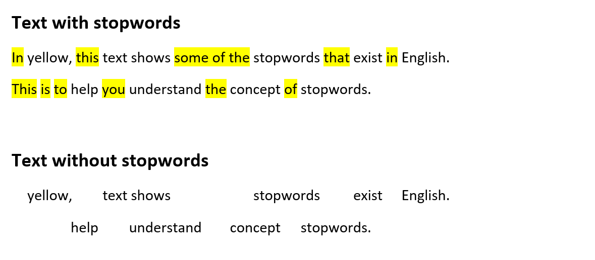
Text often contains words that hold no particular meaning. These are called stopwords and can be found throughout the text. Since stopwords rarely contribute to the understanding of the text, it is a good idea to remove them before analysing the text.
Example of removing stopwords
Tidytext and tokenisation
In the following we will be making the text machine-readable by means of the tidy text principles.
Tidy text
The tidy text princples were developed by Silge and Robinson and apply the principles from the tidy data on text.
The tidy data framework principles are:
- Each variable forms a column.
- Each observation forms a row.
- Each type of observational unit forms a table.
Applying these principles to text data leads to a format that is easily manipulated, visualised and analysed using standard data science tools.
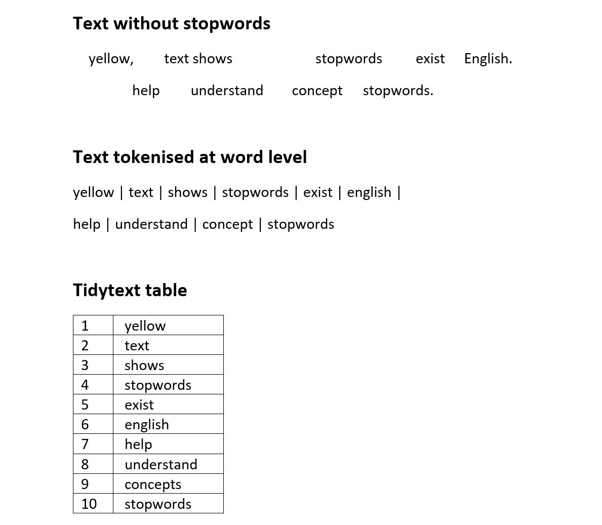
Tidy text represents the text by breaking it down into smaller parts such as sentences, words or letters. This process is called tokenisation.
Tokenisation is language independent, as long as the language uses a space between each word.
Here is an example of tokenisation at word-level.
Example of tokenization
- Know what text mining is
- Know what stopwords are
- Knowledge of the data we are working with
- Know what tidy text means
Content from Loading data
Last updated on 2026-08-18 | Edit this page
Estimated time: 0 minutes
Overview
Questions
- Which packages are needed?
- How is the dataset loaded?
- How is a dataset inspected?
Objectives
- Knowledge of the relevant packages
- Ability to to load the dataset
- Ability to inspect the dataset
Getting started
When performing text analysis in R, the built-in functions in R are
not sufficient. It is therefore necessary to install some additional
packages. In this course we will be using the packages
tidyverse, tidytext and tm.
R
install.packages("tidyverse")
install.packages("tidytext")
install.packages("tm")

library(tidyverse)
library(tidytext)
library(tm)
Getting data
Begin by downloading the dataset called articles.csv.
Place the downloaded file in the data/ folder. You can do this directly
from R by copying and pasting this into your console. (The console is
the panel under your script).
R
download.file("https://raw.githubusercontent.com/KUBDatalab/R-textmining_new/main/episodes/data/guardianArticles.csv", "data/guardianArticles.csv", mode = "wb")
After downloading the data, it needs to be loaded into R’s memory by
means of the function read_csv().
R
articles <- read_csv("data/guardianArticles.csv", na = c("NA", "NULL", ""))
Taking a first look at the dataset
R
articles
OUTPUT
# A tibble: 1,898 × 7
      id date    text                            section region author wordcount
   <dbl> <chr>   <chr>                           <chr>   <chr>  <chr>      <dbl>
 1     1 2026-05 Britain’s biometrics watchdogs… News    UK     Jessi…      1328
 2     2 2026-02 Iran’s architecture of interne… News    UK     Aisha…       657
 3     3 2026-01 TikTok will begin to roll out … News    UK     Mark …       623
 4     4 2026-05 The parent company of Donald T… News    US     Edwar…       348
 5     5 2026-05 It is a familiar story. Extrav… Opinion UK     Edito…       585
 6     6 2026-04 Sonia Bompastor, the Chelsea h… Sport   UK     Tom G…       468
 7     7 2026-03 Transcription ends with an epi… Arts    UK     Sukhd…       917
 8     8 2026-04 When Greg Swann was appointed … Sport   AUS    Jonat…       794
 9     9 2026-02 Immigration and Customs Enforc… News    US     Harry…       915
10    10 2026-01 Gathering Summer after summer,… News    UK     Rebec…      4213
# ℹ 1,888 more rows
Data description
The dataset contains newspaper articles from the Guardian newspaper. The harvested articles were published between June 2025 and May 2026 and contain the word “technology”.
The original dataset contained some variables considered irrelevant within the parameters of this course. The following variables were kept:
- id - unique number identifying each article
- date - month and publication year
- text - full text from the article
- section - Guardian news section
- region - production region
- author - name(s) of journalist(s)
- wordcount - number of words
Taking a quick look at the data
The tidyverse-package has some functions that allow you
to inspect the dataset. Below, you can see some of these functions and
what they do.
R
head(articles)
OUTPUT
# A tibble: 6 × 7
     id date    text                             section region author wordcount
  <dbl> <chr>   <chr>                            <chr>   <chr>  <chr>      <dbl>
1     1 2026-05 Britain’s biometrics watchdogs … News    UK     Jessi…      1328
2     2 2026-02 Iran’s architecture of internet… News    UK     Aisha…       657
3     3 2026-01 TikTok will begin to roll out n… News    UK     Mark …       623
4     4 2026-05 The parent company of Donald Tr… News    US     Edwar…       348
5     5 2026-05 It is a familiar story. Extrava… Opinion UK     Edito…       585
6     6 2026-04 Sonia Bompastor, the Chelsea he… Sport   UK     Tom G…       468
R
tail(articles)
OUTPUT
# A tibble: 6 × 7
     id date    text                             section region author wordcount
  <dbl> <chr>   <chr>                            <chr>   <chr>  <chr>      <dbl>
1  4970 2025-07 "[Where’s the game at?] Definit… Sport   UK     James…      8817
2  4975 2025-06 "Tim Henman, who was disqualifi… Sport   UK     Katy …      7537
3  4981 2025-06 "Ali Martin’s report will be wi… Sport   UK     Rob S…      8874
4  4994 2025-06 "An epic tie-break to end an ep… Sport   UK     John …      9208
5  5003 2025-11 "Don’t you just love Christmas … Lifest… UK     Hanna…     13325
6 5018 2025-07 "Here’s Ewan Murray’s report an… Sport UK David… 14350R
glimpse(articles)
OUTPUT
Rows: 1,898
Columns: 7
$ id        <dbl> 1, 2, 3, 4, 5, 6, 7, 8, 9, 10, 11, 12, 13, 14, 15, 16, 17, 1…
$ date      <chr> "2026-05", "2026-02", "2026-01", "2026-05", "2026-05", "2026…
$ text      <chr> "Britain’s biometrics watchdogs have warned that national ov…
$ section   <chr> "News", "News", "News", "News", "Opinion", "Sport", "Arts", …
$ region    <chr> "UK", "UK", "UK", "US", "UK", "UK", "UK", "AUS", "US", "UK",…
$ author    <chr> "Jessica Murray and Robert Booth", "Aisha Down", "Mark Swene…
$ wordcount <dbl> 1328, 657, 623, 348, 585, 468, 917, 794, 915, 4213, 1304, 66…R
names(articles)
OUTPUT
[1] "id"        "date"      "text"      "section"   "region"    "author"
[7] "wordcount"R
dim(articles)
OUTPUT
[1] 1898 7- Packages must be installed and loaded
- The dataset needs to be loaded
- The dataset can be inspected by means of different functions
Content from Tokenisation and stopwords
Last updated on 2026-08-18 | Edit this page
Estimated time: 0 minutes
Overview
Questions
- How is text prepared for analysis?
Objectives
- Ability to tokenise a text
- Ability to remove stopwords from text
Tokenisation
Since we are working with text mining, we focus on the
text coloumn. We do this because the coloumn contains the
text from the articles in question.
To tokenise a column, we use the functions
unnest_tokens() from the tidytext-package. The
function gets two arguments. The first one is word. This
defines that the text should be split up by words. The second argument,
text, defines the column that we want to tokenise.
R
articles_tidy <- articles |>
  unnest_tokens(word, text)
articles_tidy
OUTPUT
# A tibble: 2,405,300 × 7
      id date    section region author                          wordcount word
   <dbl> <chr>   <chr>   <chr>  <chr>                               <dbl> <chr>
 1     1 2026-05 News    UK     Jessica Murray and Robert Booth      1328 brita…
 2     1 2026-05 News    UK     Jessica Murray and Robert Booth      1328 biome…
 3     1 2026-05 News    UK     Jessica Murray and Robert Booth      1328 watch…
 4     1 2026-05 News    UK     Jessica Murray and Robert Booth      1328 have
 5     1 2026-05 News    UK     Jessica Murray and Robert Booth      1328 warned
 6     1 2026-05 News    UK     Jessica Murray and Robert Booth      1328 that
 7     1 2026-05 News    UK     Jessica Murray and Robert Booth      1328 natio…
 8     1 2026-05 News    UK     Jessica Murray and Robert Booth      1328 overs…
 9     1 2026-05 News    UK     Jessica Murray and Robert Booth      1328 of
10     1 2026-05 News    UK     Jessica Murray and Robert Booth      1328 ai
# ℹ 2,405,290 more rowsTokenisation
The result of the tokenisation is 2,405,300 rows. The reason is that
the text-column has been replaced by a new column named
word. This column contains all words found in all of the
articles. The information from the remaining columns is kept. This makes
is possible to determine which article each word belongs to. The reason
the data set contains so many more rows is that each word is on a row of
its own.
Stopwords
The next step is to remove stopwords. We have chosen to use the
stopword list from the package tidytext. The list contains
1,149 words that are considered stopwords. Other lists are available,
and they differ in terms of how many words they contain.
R
data(stop_words)
stop_words
OUTPUT
# A tibble: 1,149 × 2
   word        lexicon
   <chr>       <chr>
 1 a           SMART
 2 a's         SMART
 3 able        SMART
 4 about       SMART
 5 above       SMART
 6 according   SMART
 7 accordingly SMART
 8 across      SMART
 9 actually    SMART
10 after       SMART
# ℹ 1,139 more rowsAdding and removing stopwords
You may find yourself in need of either adding or removing words from the stopwords list.
Here is how you add and remove stopwords to a predefined list.
First, create a tibble with the word you wish to add to the stopwords list
R
new_stop_words <- tibble(
  word = c("cat", "dog"),
  lexicon = "my_stopwords"
)
Then make a new stopwords tibble based on the original one, but with the new words added.
R
updated_stop_words <- stop_words |>
  bind_rows(new_stop_words)
Run the following code to see that the added lexicon
my_stopwords contains two words.
R
updated_stop_words |>
  count(lexicon)
OUTPUT
# A tibble: 4 × 2
  lexicon          n
  <chr>        <int>
1 SMART          571
2 my_stopwords     2
3 onix           404
4 snowball 174First, create a vector with the word(s) you wish to remove from the stopwords list.
R
words_to_remove <- c("cat", "dog")
Then remove the rows containing the unwanted words.
R
updated_stop_words <- stop_words |>
  filter(!word %in% words_to_remove)
Run the following code to see that the added lexicon
my_stopwords nolonger exists.
R
updated_stop_words |>
  count(lexicon)
OUTPUT
# A tibble: 3 × 2
  lexicon      n
  <chr>    <int>
1 SMART      571
2 onix       404
3 snowball   174
In order to remove stopwords from articles_tidy, we have
to use the anti_join-function.
R
articles_anti_join <- articles_tidy |>
  anti_join(stop_words, by = "word")
articles_anti_join
OUTPUT
# A tibble: 1,118,028 × 7
      id date    section region author                          wordcount word
   <dbl> <chr>   <chr>   <chr>  <chr>                               <dbl> <chr>
 1     1 2026-05 News    UK     Jessica Murray and Robert Booth      1328 brita…
 2     1 2026-05 News    UK     Jessica Murray and Robert Booth      1328 biome…
 3     1 2026-05 News    UK     Jessica Murray and Robert Booth      1328 watch…
 4     1 2026-05 News    UK     Jessica Murray and Robert Booth      1328 warned
 5     1 2026-05 News    UK     Jessica Murray and Robert Booth      1328 natio…
 6     1 2026-05 News    UK     Jessica Murray and Robert Booth      1328 overs…
 7     1 2026-05 News    UK     Jessica Murray and Robert Booth      1328 ai
 8     1 2026-05 News    UK     Jessica Murray and Robert Booth      1328 power…
 9     1 2026-05 News    UK     Jessica Murray and Robert Booth      1328 scann…
10     1 2026-05 News    UK     Jessica Murray and Robert Booth      1328 catch
# ℹ 1,118,018 more rows
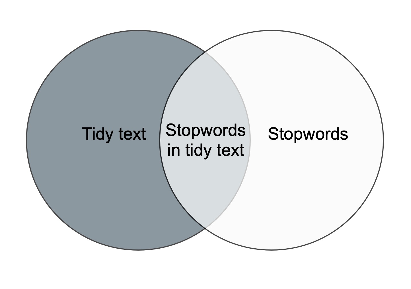
The anti_join-function removes the stopwords from the
orginal dataset. This is illustrated in the figure below. The only part
left after anti-joining is the dark grey area to the left.
These words are saved as the object
articles_anti_join.
- Know how to prepare text for analysis
Content from Word frequency analysis
Last updated on 2026-08-18 | Edit this page
Estimated time: 0 minutes
Overview
Questions
- How is a frequency analysis conducted?
Objectives
- Learn how to find frequent words
- Learn how to analyse and visualise it
Frequency analysis
A word frequency is a relatively simple analysis. It measures how often words occur in a text.
R
articles_anti_join |>
  count(word, sort = TRUE)
OUTPUT
# A tibble: 68,899 × 2
   word           n
   <chr>      <int>
 1 it’s        6584
 2 ai          5778
 3 people      4422
 4 time        4277
 5 technology  3946
 6 world       2758
 7 don’t       2131
 8 day         1803
 9 life        1694
10 uk          1690
# ℹ 68,889 more rows
The previous code chunk resulted in a list containing the most frequent words. The words are from articles about both presidents, and they are ordered by frequency with the highest number on top.
A closer look at the list may reveal that some words are irrelevant. Given that the articles in the dataset are about the two presidents’ respective inaugurations, we consider the words below irrelevant for our analysis. Therefore, we make a new dataset without these words.
Notice that the we use a “!” as part of the filter function. By doing that, we filter on anything but the words inside the parenthesis.
R
articles_filtered <- articles_anti_join |>
  filter(!word %in% c("it’s", "don’t"))

articles_filtered |>
  count(word, sort = TRUE)
OUTPUT
# A tibble: 68,897 × 2
   word           n
   <chr>      <int>
 1 ai          5778
 2 people      4422
 3 time        4277
 4 technology  3946
 5 world       2758
 6 day         1803
 7 life        1694
 8 uk          1690
 9 that’s      1667
10 government  1644
# ℹ 68,887 more rows
The words deemed irrelevant are no longer on the list above.
Instead of a general list it may be more interesting to focus on the most frequent words in certain sections from The Guardian.
R
articles_filtered |>
  count(section, word, sort = TRUE)
OUTPUT
# A tibble: 138,065 × 3
   section   word           n
   <chr>     <chr>      <int>
 1 News      ai          3131
 2 News      technology  1993
 3 Sport     england     1371
 4 Sport     ball        1287
 5 Opinion   ai          1250
 6 Sport     1           1239
 7 News      people      1196
 8 Lifestyle time        1117
 9 Lifestyle people      1062
10 Sport     time        1050
# ℹ 138,055 more rows
Keeping an overview of the words associated with each section can be a bit tricky. For instance, the word “time” is associated with both lifestyle and sport.
Another way of comparing words across different sections could by counting them per section. In the example below, the section is the guiding principle.
R
articles_filtered |>
  count(section, word, sort = TRUE) |>
  pivot_wider(
    names_from = section,
    values_from = n
  )
OUTPUT
# A tibble: 68,897 × 6
   word        News Sport Opinion Lifestyle  Arts
   <chr>      <int> <int>   <int>     <int> <int>
 1 ai          3131    36    1250       351  1010
 2 technology  1993   294     565       466   628
 3 england      106  1371      41        27    47
 4 ball           5  1287      11        40    20
 5 1             89  1239      40       106    73
 6 people      1196   250     883      1062  1031
 7 time         676  1050     551      1117   883
 8 government  1024    19     429        65   107
 9 2             68   968      25       161   119
10 game          25   953      31       144   386
# ℹ 68,887 more rows
Proportion
Simply counting the words does not give us any information about proportional distribution. For instance, in the AI row, we do not know if the 3131 ocurrences of AI in the news is a lot compared to the 1250 ocurrences in the opinion section.
Therefore, let us have a look at how it looks if we make the same query, but with proportion insted of word count.
R
articles_filtered |>
  count(section, word) |>
  group_by(section) |>
  mutate(proportion = n / sum(n)) |>
  ungroup() |>
  select(-n) |>
  arrange(desc(proportion)) |>
  pivot_wider(
    names_from = section,
    values_from = proportion)
OUTPUT
# A tibble: 68,897 × 6
   word            News   Opinion    Sport      Arts Lifestyle
   <chr>          <dbl>     <dbl>    <dbl>     <dbl>     <dbl>
 1 ai         0.0125    0.00809   0.000175 0.00450   0.00128
 2 technology 0.00795   0.00366   0.00143  0.00280   0.00170
 3 england    0.000423  0.000265  0.00668  0.000209  0.0000984
 4 ball       0.0000199 0.0000712 0.00627  0.0000891 0.000146
 5 1          0.000355  0.000259  0.00604  0.000325  0.000386
 6 people     0.00477   0.00571   0.00122  0.00459   0.00387
 7 time       0.00270   0.00357   0.00512  0.00393   0.00407
 8 2          0.000271  0.000162  0.00472  0.000530  0.000587
 9 game       0.0000997 0.000201  0.00465  0.00172   0.000525
10 australia  0.00106   0.000912  0.00417  0.000401  0.000153
# ℹ 68,887 more rows
Visualization
We can also visualize word frequency. Below is a visualisation of the 10 most frequent words in each section. The plots do not contain information about proportions, though the x-axis does give us information about the size of each section.
R
articles_filtered |>
  group_by(section) |>
  count(word, sort = TRUE) |>
  top_n(10) |>
  ungroup() |>
  mutate(word = reorder_within(word, n, section)) |>
  ggplot(aes(n, word, fill = section)) +
  geom_col() +
  facet_wrap(~section, scales = "free") +
  scale_y_reordered() +
  labs(x = "word occurrences")
OUTPUT
Selecting by n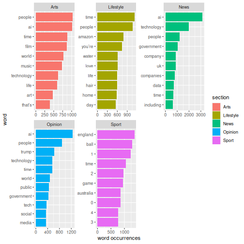
A close look at the plot belonging to the Sport section reveals that
numbers occur five times. In order to find out what is behind these
numbers, we have to return to the original dataset
articles. The reason we have to use the original dataset is
that it still has the intact text. Below, we investigate which words
sorround the number “1”.
For this purpose we need a package named
quanteda. First, the package is installed, and then it is
activated.
R
install.packages("quanteda")
library(quanteda)
To get the context, we use the function kwic.
R
articles_context <- articles |>
  filter(section == "Sport") |>
  # filter(str_detect(text, "\\b1\\b")) |>
  # slice(1) |>
  pull(text) |>
  tokens() |>
  kwic(pattern = "1", window = 10)

articles_context |> head()
OUTPUT
Keyword-in-context with 6 matches.

   [text4, 270] and Emma Raducanu, the men’s and women’s British No | 1 |
  [text40, 377]                 ), 6-3 win in front of a roaring No | 1 |
   [text43, 28]               not “ 100% accurate ”. The British No | 1 |
  [text51, 785]        court, contended Jane Carter, 58, outside No | 1 |
  [text51, 850]     down the game. Standing beneath the shade of No | 1 |
 [text52, 2416]                he said. “ I would have been your No | 1 |

 players, who each criticised the ELC system following their
 Court crowd. Spectators appeared to boo Jarry when the
 said it was “ a shame ” human line judges
 Court. “ I would think that it would improve
 Court, Tom Mansell said the technology takes the “
 proponent after Joe Biden. ” The former president is
We are looking for at keyword in context, and this is exactly what
the function kwic does. It locates the string we write in
the argument pattern and takes the amount of words before
and after the keyword given in the argument window. In this
case the number of words before and after “1” is set to 10.
It may be worth saving the result, so that it can be analysed further. One way of doing this is by saving it as a csv-file.
- Making a frequency analysis
- Visualising the results
Content from Sentiment analysis
Last updated on 2026-08-18 | Edit this page
Estimated time: 0 minutes
Overview
Questions
- What is a sentiment?
- How is sentiment analysis conducted?
Objectives
- Learn about different lexicons
- Learn how to add sentiment to words using lexicons
- Analyse and visualise the sentiments in a text
Sentiment analysis
Sentiment refers to the emotion or tone in a text. It is typically categorised as positive, negative or neutral. Sentiment is often used to analyse opinions, attitudes or emotions in written content. In this case the written content is newspaper articles.
Sentiment analysis is a method used to identify and classify emotions in textual data. This is often done using word list (lexicons). The goal is to determine whether a given text has a positive, negative or neutral tone.
In order to do a sentiment analysis on our data we From the previous section we have a dataset containing a list of words in the text without stopwords. To do a sentiment analysis we can use a so-called lexicon and assign a sentiment to each word. In order to do this we need an list of words and their sentiment. A simple form would be wether they are positive or negative.
There are multiple sentiment lexicons. For a start we will be using
the bing lexicon. This lexicon categorizes words as either
positive or negative.
R
get_sentiments("bing")
OUTPUT
# A tibble: 6,786 × 2
   word        sentiment
   <chr>       <chr>
 1 2-faces     negative
 2 abnormal    negative
 3 abolish     negative
 4 abominable  negative
 5 abominably  negative
 6 abominate   negative
 7 abomination negative
 8 abort       negative
 9 aborted     negative
10 aborts      negative
# ℹ 6,776 more rows
In order to use the bing-lexicon, we have to save
it.
R
bing <- get_sentiments("bing")
We now need to combine the sentiment with the words from the articles. This is done by performing an inner_join.
R
articles_bing <- articles_filtered |>
  inner_join(bing)
OUTPUT
Joining with `by = join_by(word)`R
articles_bing
OUTPUT
# A tibble: 123,667 × 8
      id date    section region author                 wordcount word  sentiment
   <dbl> <chr>   <chr>   <chr>  <chr>                      <dbl> <chr> <chr>
 1     1 2026-05 News    UK     Jessica Murray and Ro…      1328 warn… negative
 2     1 2026-05 News    UK     Jessica Murray and Ro…      1328 over… negative
 3     1 2026-05 News    UK     Jessica Murray and Ro…      1328 lagg… negative
 4     1 2026-05 News    UK     Jessica Murray and Ro…      1328 rapid positive
 5     1 2026-05 News    UK     Jessica Murray and Ro…      1328 slow  negative
 6     1 2026-05 News    UK     Jessica Murray and Ro…      1328 warn… negative
 7     1 2026-05 News    UK     Jessica Murray and Ro…      1328 effe… positive
 8     1 2026-05 News    UK     Jessica Murray and Ro…      1328 misu… negative
 9     1 2026-05 News    UK     Jessica Murray and Ro…      1328 over… negative
10     1 2026-05 News    UK     Jessica Murray and Ro…      1328 brea… positive
# ℹ 123,657 more rows
In R, inner_join() is commonly used to combine datasets
based on a shared column. In this case it is the word
column. inner_join() matches words from a text dataset, in
this case articles_filtered with words in the Bing
sentiment lexicon to determine whether they are positive or
negative.
Once we have the combined dataset we can make a sentiment analysis. A way to start could be by counting the number of positive and negative words used in the articles. This is done per section.
R
articles_bing |>
  group_by(section) |>
  summarise(positive = sum(sentiment == "positive"),
            negative = sum(sentiment == "negative"),
            difference = positive - negative)
OUTPUT
# A tibble: 5 × 4
  section   positive negative difference
  <chr>        <int>    <int>      <int>
1 Arts         11844    13555      -1711
2 Lifestyle    18337    13504       4833
3 News         11216    14220      -3004
4 Opinion       8452    11419      -2967
5 Sport        11350     9770       1580
The result shows the distribution of positive and negative words across sections. It also shows that Lifestyle has the highest number of positive words, and that oponion has the highest number of negative words. The section with the lowest difference is Arts.
Another way of presenting this analysis is by visualising it.
R
articles_bing |>
  group_by(section, date) |>
  summarise(positive = sum(sentiment == "positive"),
            negative = sum(sentiment == "negative"),
            difference = positive - negative) |>
  #ungroup() |>
  filter(section %in% c("Arts", "Sport")) |>
  ggplot(mapping = aes(x = date, y = difference, colour = section, group = section)) +
  geom_point() +
  geom_line()
OUTPUT
`summarise()` has regrouped the output.
ℹ Summaries were computed grouped by section and date.
ℹ Output is grouped by section.
ℹ Use `summarise(.groups = "drop_last")` to silence this message.
ℹ Use `summarise(.by = c(section, date))` for per-operation grouping
  (`?dplyr::dplyr_by`) instead.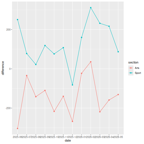
By looking at the graphs, we can see that the wording in December in Sport articles is quite negative compared to February. If we had a data set covering more years it would be worth investigating if this was a tendency or just a coincidence.
For now, it might be interesting to read the articles from December and February in order to compare their content. To that end we can create a new dataset containing articles from the Sport section from December and February.
R
interesting_articles <- articles |>
  filter(section == "Sport") |>
  filter(date %in% c("2025-12", "2026-02"))
This can be saved as csv-file for further analysis.
R
write_csv(interesting_articles, "data_out/interesting_articles.csv")
With bing we only look at the sentiment in a binary
fashion - a word is either positive or negative. If we do a similar
analysis with AFINN, it looks different. Like
bing, AFINN is a sentiment lexicon. It
consists of a list of words that are assigned sentiment scores ranging
from -5 (very negative) to +5 (very positive). Note that
AFINN does not contain a 0.
AFINN is part of the package textdata, so
we need to install the package and run the library in order to be able
to use it in this script.
R
install.packages("textdata")
library(textdata)
So that we can use the AFINN-lexicon, we have to save
it.
R
afinn <- get_sentiments("afinn")
This is what it looks like.
R
afinn
OUTPUT
# A tibble: 2,477 × 2
   word       value
   <chr>      <dbl>
 1 abandon       -2
 2 abandoned     -2
 3 abandons      -2
 4 abducted      -2
 5 abduction     -2
 6 abductions    -2
 7 abhor         -3
 8 abhorred      -3
 9 abhorrent     -3
10 abhors        -3
# ℹ 2,467 more rowsBemærk at vi ikke på github kan downloade afinn. Derfor har vi downloaded afinn datasættet til en csv-fil pr 21. november 2025. Med andre ord er der risiko for at siden kører med et uopdateret datasæt. - TROR IKKE VI BEHØVER DET MERE - SNAK MED CHRISTIAN
We now need to combine the sentiment to the words from our articles. We do this by performing an inner_join.
R
articles_afinn <- articles_filtered |>
  inner_join(afinn)
OUTPUT
Joining with `by = join_by(word)`Since the AFINN lexicon ascribes either negative or
positive numbers each word (instead of strings, as bing
does),we can easily calculate the difference as we did with
bing.
R
articles_afinn |>
  group_by(section) |>
  summarise(different = sum(value))
OUTPUT
# A tibble: 5 × 2
  section   different
  <chr>         <dbl>
1 Arts            730
2 Lifestyle     11230
3 News          -5744
4 Opinion       -4335
5 Sport          8045
It could be interesting to see how the different levels of negative and positive words are used in the different sections.
R
articles_afinn |>
  #group_by(section) |>
  count(section, value) |>
  pivot_wider(names_from = value, values_from = n)
OUTPUT
# A tibble: 5 × 11
  section    `-5`  `-4`  `-3`  `-2`  `-1`   `1`   `2`   `3`   `4`   `5`
  <chr>     <int> <int> <int> <int> <int> <int> <int> <int> <int> <int>
1 Arts         14   203  2122  4807  2718  3189  4287  2037   574    28
2 Lifestyle     3   130  1444  4139  3560  5126  6468  2683   416    32
3 News          1    94  2283  6081  3860  4917  4922   699   155     6
4 Opinion       7    72  1802  4549  2496  2963  3610   721   153     6
5 Sport         9    52  1123  3563  2598  2871  3859  1894  1195    68
This is what it looks like if we add proportions to the calculation.
R
articles_afinn |>
  count(section, value) |>
  group_by(section) |>
  mutate(proportion = n / sum(n)) |>
  ungroup() |>
  select(-n) |>
  #arrange(desc(proportion)) |>
  pivot_wider(names_from = value, values_from = proportion)
OUTPUT
# A tibble: 5 × 11
  section     `-5`    `-4`   `-3`  `-2`  `-1`   `1`   `2`    `3`     `4`     `5`
  <chr>      <dbl>   <dbl>  <dbl> <dbl> <dbl> <dbl> <dbl>  <dbl>   <dbl>   <dbl>
1 Arts     7.01e-4 0.0102  0.106  0.241 0.136 0.160 0.215 0.102  0.0287  1.40e-3
2 Lifesty… 1.25e-4 0.00542 0.0602 0.172 0.148 0.214 0.269 0.112  0.0173  1.33e-3
3 News     4.34e-5 0.00408 0.0992 0.264 0.168 0.214 0.214 0.0304 0.00673 2.61e-4
4 Opinion  4.27e-4 0.00440 0.110  0.278 0.152 0.181 0.220 0.0440 0.00934 3.66e-4
5 Sport    5.22e-4 0.00302 0.0652 0.207 0.151 0.167 0.224 0.110  0.0693  3.95e-3
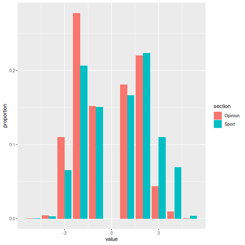
If we focus on the two sections Sport and Opinion, this is what it
looks like when we visualise it by means of ggplot().
R
articles_afinn |>
  count(section, value) |>
  group_by(section) |>
  mutate(proportion = n / sum(n)) |>
  ungroup() |>
  select(-n) |>
  filter(section %in% c("Sport", "Opinion"))  |>
  ggplot(mapping = aes(x = value, y = proportion, fill = section)) +
  geom_col(position = "dodge")
n-grams and correlations
So far we have been looking at words as individual units and not considered how they are related to the other words around them. It is possible to conduct an analysis that looks at the relationsships between words in our text.
Instead of using the unnest_tokens-function at singular
word level, as we have done so far, we will tokenize our text in to
sequences of words. These sequences are called n-grams. They allow us to
see how often a word is followed by another word. This gives us a chance
to look at the relationsship between words.
We no longer want to use articles_filteres, since this
has been tokenized word by word. We need a dataframe where
each article text is in a cell of its own. Therefore, we will go back to
our orginal object articles that contains all the articles
in their original state.
First we tokenise the text so that each cell contains two words.
R
articles_bigrams <- articles |>
 unnest_tokens(bigram, text, token = "ngrams", n = 2) |>
 filter(!is.na(bigram))
R
articles_bigrams
OUTPUT
# A tibble: 2,403,402 × 7
      id date    section region author                          wordcount bigram
   <dbl> <chr>   <chr>   <chr>  <chr>                               <dbl> <chr>
 1     1 2026-05 News    UK     Jessica Murray and Robert Booth      1328 brita…
 2     1 2026-05 News    UK     Jessica Murray and Robert Booth      1328 biome…
 3     1 2026-05 News    UK     Jessica Murray and Robert Booth      1328 watch…
 4     1 2026-05 News    UK     Jessica Murray and Robert Booth      1328 have …
 5     1 2026-05 News    UK     Jessica Murray and Robert Booth      1328 warne…
 6     1 2026-05 News    UK     Jessica Murray and Robert Booth      1328 that …
 7     1 2026-05 News    UK     Jessica Murray and Robert Booth      1328 natio…
 8     1 2026-05 News    UK     Jessica Murray and Robert Booth      1328 overs…
 9     1 2026-05 News    UK     Jessica Murray and Robert Booth      1328 of ai
10     1 2026-05 News    UK     Jessica Murray and Robert Booth      1328 ai po…
# ℹ 2,403,392 more rows
It looks much like the result of a tokenisation at singular word level, but the added column is now called bigram and contains two words
We can now count how many times word pair occurs.
R
articles_bigrams |>
  count(bigram, sort = TRUE)
OUTPUT
# A tibble: 923,094 × 2
   bigram       n
   <chr>    <int>
 1 of the   11380
 2 in the   10393
 3 to the    5100
 4 on the    4680
 5 and the   3755
 6 at the    3717
 7 to be     3575
 8 for the   3464
 9 in a      3211
10 with the  2909
# ℹ 923,084 more rows
Here we can see that the birams that tops the list are pairs of quite common words. Many of these are words that were defined as stopwords earlier. By removing pairs that contain at least one stopwords, we get at more meaningful result.
In order to be able to remove these pairs, we have to put each word
in its own column. We can do this by using the function
separate.
First we separate each pair into two columns. We to this by using the white space between the words as a separator.
R
bigrams_separated <- articles_bigrams |>
  separate(bigram, c("word1", "word2"), sep = " ")

bigrams_separated
OUTPUT
# A tibble: 2,403,402 × 8
      id date    section region author                     wordcount word1 word2
   <dbl> <chr>   <chr>   <chr>  <chr>                          <dbl> <chr> <chr>
 1     1 2026-05 News    UK     Jessica Murray and Robert…      1328 brit… biom…
 2     1 2026-05 News    UK     Jessica Murray and Robert…      1328 biom… watc…
 3     1 2026-05 News    UK     Jessica Murray and Robert…      1328 watc… have
 4     1 2026-05 News    UK     Jessica Murray and Robert…      1328 have  warn…
 5     1 2026-05 News    UK     Jessica Murray and Robert…      1328 warn… that
 6     1 2026-05 News    UK     Jessica Murray and Robert…      1328 that  nati…
 7     1 2026-05 News    UK     Jessica Murray and Robert…      1328 nati… over…
 8     1 2026-05 News    UK     Jessica Murray and Robert…      1328 over… of
 9     1 2026-05 News    UK     Jessica Murray and Robert…      1328 of    ai
10     1 2026-05 News    UK     Jessica Murray and Robert…      1328 ai    powe…
# ℹ 2,403,392 more rows
Once that is done, we remove the rows that contain a stopword in either of the two new columns.
R
bigrams_filtered <- bigrams_separated |>
  filter(!word1 %in% stop_words$word) |>
  filter(!word2 %in% stop_words$word)

bigrams_filtered
OUTPUT
# A tibble: 479,613 × 8
      id date    section region author                     wordcount word1 word2
   <dbl> <chr>   <chr>   <chr>  <chr>                          <dbl> <chr> <chr>
 1     1 2026-05 News    UK     Jessica Murray and Robert…      1328 brit… biom…
 2     1 2026-05 News    UK     Jessica Murray and Robert…      1328 biom… watc…
 3     1 2026-05 News    UK     Jessica Murray and Robert…      1328 nati… over…
 4     1 2026-05 News    UK     Jessica Murray and Robert…      1328 ai    powe…
 5     1 2026-05 News    UK     Jessica Murray and Robert…      1328 catch crim…
 6     1 2026-05 News    UK     Jessica Murray and Robert…      1328 tech… rapid
 7     1 2026-05 News    UK     Jessica Murray and Robert…      1328 rapid grow…
 8     1 2026-05 News    UK     Jessica Murray and Robert…      1328 metr… poli…
 9     1 2026-05 News    UK     Jessica Murray and Robert…      1328 past  12
10     1 2026-05 News    UK     Jessica Murray and Robert…      1328 12    mont…
# ℹ 479,603 more rows
Now we can make a new count of word pair.
R
bigram_counts <- bigrams_filtered |>
  count(word1, word2, sort = TRUE)

bigram_counts
OUTPUT
# A tibble: 347,703 × 3
   word1      word2            n
   <chr>      <chr>        <int>
 1 social     media          760
 2 artificial intelligence   392
 3 world      cup            293
 4 chief      executive      256
 5 donald     trump          243
 6 tech       companies      235
 7 south      africa         230
 8 premier    league         207
 9 final      cut            198
10 facial     recognition    191
# ℹ 347,693 more rows
This gives us a more meaningful set of word pairs.
If we want to combine the colums again, so that the words pairs
(without stopwords) are back in the same column, it can easily be done
by using the function unite
R
bigrams_united <- bigrams_filtered |>
  unite(bigram, word1, word2, sep = " ")

bigrams_united
OUTPUT
# A tibble: 479,613 × 7
      id date    section region author                          wordcount bigram
   <dbl> <chr>   <chr>   <chr>  <chr>                               <dbl> <chr>
 1     1 2026-05 News    UK     Jessica Murray and Robert Booth      1328 brita…
 2     1 2026-05 News    UK     Jessica Murray and Robert Booth      1328 biome…
 3     1 2026-05 News    UK     Jessica Murray and Robert Booth      1328 natio…
 4     1 2026-05 News    UK     Jessica Murray and Robert Booth      1328 ai po…
 5     1 2026-05 News    UK     Jessica Murray and Robert Booth      1328 catch…
 6     1 2026-05 News    UK     Jessica Murray and Robert Booth      1328 techn…
 7     1 2026-05 News    UK     Jessica Murray and Robert Booth      1328 rapid…
 8     1 2026-05 News    UK     Jessica Murray and Robert Booth      1328 metro…
 9     1 2026-05 News    UK     Jessica Murray and Robert Booth      1328 past …
10     1 2026-05 News    UK     Jessica Murray and Robert Booth      1328 12 mo…
# ℹ 479,603 more rows
Now we can seee how different word pairs, are used in different sections.
R
bigrams_united |>
  count(section, bigram, sort = TRUE) |>
  pivot_wider(
    names_from = section,
    values_from = n)
OUTPUT
# A tibble: 347,703 × 6
   bigram                   News Sport Lifestyle Opinion  Arts
   <chr>                   <int> <int>     <int>   <int> <int>
 1 social media              284    36       128     174   138
 2 world cup                   2   284        NA      NA     7
 3 artificial intelligence   262     5        12      64    49
 4 south africa                8   209         2       3     8
 5 premier league              1   203         2      NA     1
 6 final cut                  NA    NA       197      NA     1
 7 chief executive           186    23        17       9    21
 8 john lewis                  3    NA       169       1    10
 9 facial recognition        159    NA         1      26     5
10 tech companies            155    NA         5      57    18
# ℹ 347,693 more rows
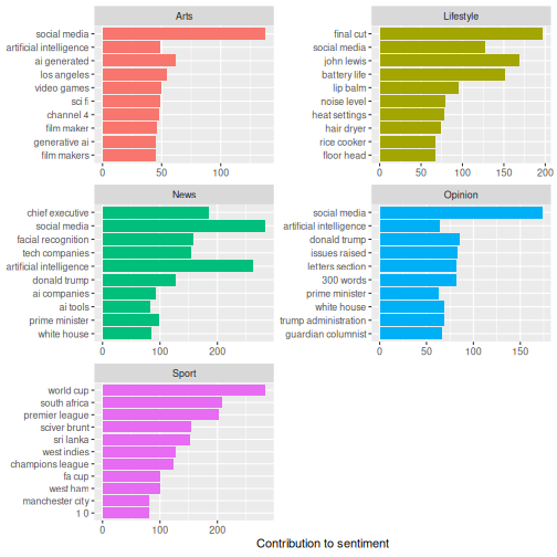
We could also have a look at the 10 most used bigrams in the different sections.
R
bigrams_united |>
  count(section, bigram, sort = TRUE) |>
  #ungroup() |>
  group_by(section) |>
  slice_max(n, n = 10) |>
  ungroup() |>
  mutate(bigram = reorder(bigram, n)) |>
  ggplot(mapping = aes(x = n, y = bigram, fill = section)) +
  geom_col(show.legend = FALSE) +
  facet_wrap(~section, scales = "free", ncol = 2) +
  labs(x = "Contribution to sentiment",
       y = NULL)
- Sentiments is the emotion or tone in a text
- There are different lexicons
- It is possible to add sentiments to words
- It is possible to visualise the sentiments
- It is possible to look at relationsship between words
Content from Whats next?
Last updated on 2026-08-18 | Edit this page
Estimated time: 12 minutes
Overview
Questions
- What is the next step?
Objectives
- Explain how to use markdown with the new lesson template
- Demonstrate how to include pieces of code, figures, and nested challenge blocks
For general techniques and approaches to working with text in a tidy manner, we recommend the Text Mining with R book by Julia Silge and David Robinson.
Julia Silge have her own youtube channel where she, among other things, do text analysis. You will learn a lot by listening to her thoughts while she code.
Text can be found everywhere. Rather than scraping text yourself, you can find R-packages containing text.
janeaustenr contains the text of Jane Austens novels.
Get it by running install.packages("janeaustenr")
The sherlock package contains the complete Sherlock
Holmes collection by Arthur Conan Doyle. It must be installed from
github, running
devtools::install_github("EmilHvitfeldt/sherlock").
- Use
.mdfiles for episodes when you want static content - Use
.Rmdfiles for episodes when you need to generate output - Run
sandpaper::check_lesson()to identify any issues with your lesson - Run
sandpaper::build_lesson()to preview your lesson locally