Episode 3 word frequency analysis

Overview

Teaching: 0 min
Exercises: 0 min

Questions

How can we find the most frequent terms from each party?

Objectives

Learning how to analyze term frequency and visualize it

R Markdown

library(tidyverse)
library(tidytext)
library(tm)

Word frequency

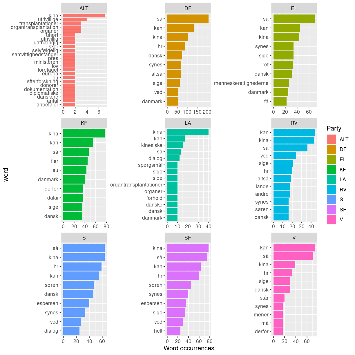
Now that we have seen the average sentiment of the parties, we want to get a deeper understanding of what they talk about when discussing China. We can calculate the most frequent words that each party uses, and then visualize that to get an impression of what they talk about when discussing China.

First we calculate the 10 most frequent words that each party says

kina_top_10_ord <- kina_tidy_blokke %>% 
  filter(Role != "formand") %>% 
  group_by(Party) %>% 
  count(word, sort = TRUE) %>%
  top_n(10) %>% 
  ungroup() %>% 
  mutate(word = reorder_within(word, n, Party))

Selecting by n

Now we want to visualize the result

kina_top_10_ord %>% 
  ggplot(aes(n, word, fill = Party)) +
  geom_col() + 
  facet_wrap(~Party, scales = "free") +
  scale_y_reordered() +
  labs(x = "Word occurrences")

plot of chunk unnamed-chunk-5

A more extensive stopword list for Danish is the ISO stopword list. We will use it know, so lets download it from the repository. Then we save it as an object. Then we make it into a tibble to prepare it for anti_join with our dataset

download.file("https://raw.githubusercontent.com/KUBDatalab/R-textmining/main/data/iso_stopwords.csv", "data/iso_stopwords.csv", mode = "wb")

iso_stopwords <- read_csv("data/iso_stopwords.csv")

Let us now apply it to the dataset by anti_join

kina_top_10_ord_2 <- kina_tidy_blokke %>% 
  anti_join(iso_stopwords, by = "word")

Unfortunately for us, most of the most common words are words that act like stopwords, carrying no meaning in themselves. To get around this, we can create our own custom list of stopwords as a tibble, and then anti_join it with the dataset, just like we did for the already existing stopword lists.

First we look at the top words to find the stopwords for our custom stopword list. Here I have printed 10, but I have looked at over 70

kina_top_10_ord_2 %>% 
  count(word, sort = TRUE) %>% 
  top_n(10) %>% 
  tbl_df %>% 
  print(n=10)

Selecting by n

# A tibble: 10 × 2
   word           n
   <chr>      <int>
kina         495
hr           476
dansk        278
synes        236
søren        217
ordføreren   197
danmark      193
tak          189
espersen     175
altså        160

Based on this, we select the words that we consider stopwords and make them into a tibble. We also want to include among our stopwords the word Danmark and its genitive case and derivative adjectives, because Denmark of course is frequently named in a Danish parliamentary debate and adds little to our analysis and understanding. Let’s also remove the name China, its genitive case and derivative adjectives, because we know that the debate is about China. Let’s also remove words that state the title or role of a member of the parliament. Let’s also remove the words spørgsmål and møder, as it relates internal questions and meetings among the members of parliament. Let’s also remove the words about Folketingets Præsidium, which do not pertain to the content of the debate. Upon later examinations some more names have also been added to the custom stopword list

custom_stopwords <- tibble(word = c("så", "kan", "hr", "sige", "synes", "ved", "altså", "søren", "tror", 
                                    "få", "bare", "derfor", "godt", "andre", "må", "espersen", "mener", "gøre", "helt", "dag", 
                                    "faktisk", "folkeparti", "gerne", "side", "gør", "nogen", "fordi", "hvordan", "tak",
                                    "måde", "set", "siger", "andet", "sagt", "år", "lige", "står", "tage", "nemlig", "lidt",
                                    "sag", "går", "kommer", "nok", "danmark", "danmarks", "dansk", "danske", "danskt", 
                                    "kina", "kinas", "kinesisk", "kinesiske", "kinesiskt", "kineser", "kineseren", 
                                    "kinesere", "kineserne", "ordfører", "ordføreren", "ordførerens", "ordførere", "ordførerne", 
                                    "spørgsmål", "møder", "holger", "k", "nielsen", "regering", "regeringen", "regeringens", 
                                    "folketinget", "folketingets", "måske", "forslag", "egentlig", "rigtig", "rigtigt", "rigtige", 
                                    "hvert", "bør", "grund", "vigtig", "vigtigt", "vigtige", "ting", "ønsker", "fru", "hr", 
                                    "selvfølgelig", "gange", "præcis", "sagde", "hele", "fald", "enhedslisten", "sidste", 
                                    "forstå", "betyder", "alliances", "fortsat", "venstre", "holde", "præsidium", "baseret",
                                    "lande", "land", "gjorde", "pind", "simpelt", "frem", "præsidiet", "præsidium", 
                                    "dokument", "tale", "hen", "o.k", "alverden", "angiveligt"))

We then do an anti_join of our custom stopword list to our tidy text

kina_top_10_ord_3 <- kina_top_10_ord_2 %>% 
  anti_join(custom_stopwords, by = "word")

Let’s now calculate the top 10 words from each party and save it as an object

kina_top_10_ord_4 <- kina_top_10_ord_3 %>% 
  filter(Role != "formand") %>% 
  group_by(Party) %>% 
  count(word, sort = TRUE) %>%
  top_n(10) %>% 
  ungroup() %>% 
  mutate(word = reorder_within(word, n, Party))

Selecting by n

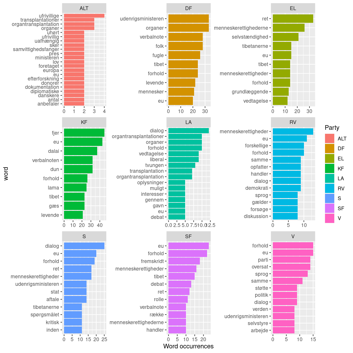
Let us now plot the result

kina_top_10_ord_4 %>% 
  ggplot(aes(n, word, fill = Party)) +
  geom_col() + 
  facet_wrap(~Party, scales = "free") +
  scale_y_reordered() +
  labs(x = "Word occurrences")

plot of chunk unnamed-chunk-14

tf_idf

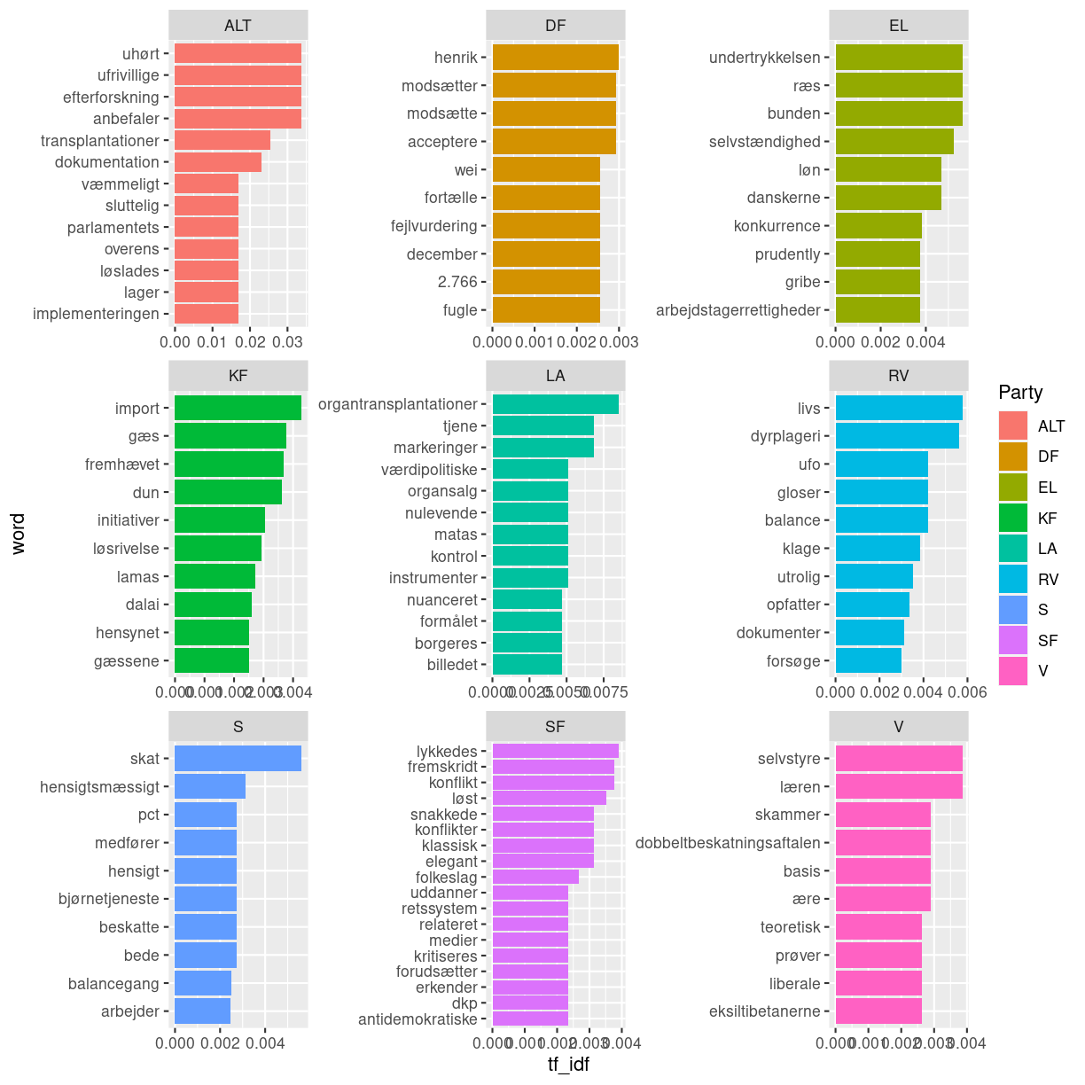
We see that many words co-occur among the parties. How can we make a plot of what each party talks about that the others don’t? We can use the tf_idf calculation. Briefly, tf_idf in this case looks at the words that occur among each party, and gives a high value to those that frequently occur in one party but rarely occur among the other parties. This will give us a sense of what each party emphasizes in their speeches about China

First we need to calculate the tf_idf of each word in our tidy text

kina_tidy_tf_idf <- kina_top_10_ord_3 %>% 
  filter(Role != "formand") %>% 
  count(Party, word, sort = TRUE) %>% 
  bind_tf_idf(word, Party, n) %>% 
  arrange(desc(tf_idf))

Now we want to select each party’s 10 words that have the highest tf_idf

kina_tidy_tf_idf_top_10 <- kina_tidy_tf_idf %>% 
  group_by(Party) %>% 
  top_n(10) %>% 
  ungroup() %>% 
  mutate(word = reorder_within(word, tf_idf, Party))

Selecting by tf_idf

Now let’s make our plot.

kina_tidy_tf_idf_top_10 %>%  
  ggplot(aes(tf_idf, word, fill = Party)) +
  geom_col() +
  facet_wrap(~Party, scales = "free") +
  scale_y_reordered() +
  labs(x = "tf_idf")

plot of chunk unnamed-chunk-17

Key Points

Custom stopword list may be necessary depending on the context

previous episode

Text mining with R

next episode