Introduction

Overview

Teaching: 0 min
Exercises: 0 min

Questions

• Key question (FIXME)

Objectives

• First learning objective. (FIXME)

FIXME

Key Points

• First key point. Brief Answer to questions. (FIXME)

Episode 1 Loading data

Overview

Teaching: 0 min
Exercises: 0 min

Questions

• What is text mining and how do we load in the dataset?

Objectives

• To be introduced to text mining and loading in text data

R Markdown

What is text mining?

Text mining refers to the use of digital tools to enable automatized analyses of text data. These analyses can enable insight into a collection of texts that can be difficult to spot with the naked eye. Furthermore, text mining tools allow the user to analyze large samples of texts and visualize the results

Installing and loading relevant libraries

We need to install some libraries that can perform the various steps in text analysis, because the base functions of R are not enough. Then we need to load them

library(tidyverse)
library(tidytext)
library(tm)

install.packages("tidyverse")
install.packages("tidytext")
install.packages("tm")
library(tidyverse)
library(tidytext)
library(tm)

Documentation for each package:

• tidyverse
• tidytext
• tm

Delimiting and loading dataset

The dataset that we will load is a collection of all debates in the Danish Parliament (Folketinget) from fall 2009 to spring 2017. In the Danish Parliament, every word from every speech in the debates is written in down in the summary. Furthermore, all speeches are described by useful and thorough metadata that allow for insightful analyses. The dataset was originally retrieved at https://repository.clarin.dk/repository/xmlui/handle/20.500.12115/44, and has been prepared for today’s course. We are going to work with a filtered dataset that contains all parliament speeches on the topic of China. Similarly, debates about any other country could have been filtered for analysis.

**The steps for delimiting the dataset were the following: We read the dataset into RStudio and saved it as a tibble

data <- read_delim(“C:/Users/swha/Desktop/Mappe/R/Tekstanalyse/Folketinget/1 fil 2009-2017/Folketingsreferater_2009_2017_samlet.txt”)

We wanted to convert the text in two of the columns to lowercase and save them in the tibble. Converting to lowercase makes filtering better, because we can find instances where the country name, which is normally in uppercase in Danish, appears as part of a compound noun or compound name, which is a common way that nouns and names are joined together to form new words and names in the Danish language data$`Agenda title` <- tolower(data$`Agenda title`) data$Text <- tolower(data$Text)

Now we needed to filter the data to speeches about China and save it as a tibble. We chose to filter on `Agenda title`, because it gives the a complete list of speeches about China. If we were to use the speech text itself, we would have missed speeches about China that did not use the the name China or its derivative adjectives, compound nouns and compound names. str_detect allows us to find instances of speeches about China where the name or the adjective appears either on its own or as part of other words

data_kina <- data %>% 
  filter(
    str_detect(`Agenda title`, "kina") | str_detect(`Agenda title`, "kines")
  )

To check that all the speeches relate to China, we wanted to have a list of all the different `Agenda title`s in the filtered data

unique(data_kina$`Agenda title`)

We saw that one of the `Agenda title`s had the work “maskinarbejder” in it. The speeches on this `Agenda title` obviously don’t relate to China, so we filter the speeches on this `Agenda title` away

data_kina <- data_kina %>% 
  filter(
    !str_detect(`Agenda title`, "maskinarbejder")
  ) 

Now that the dataset was properly filtered to parliament speeches about China, we wrote it as a txt.-file, so that it can easily be loaded into RStudio by you

library(tidyverse)

kina <- read_delim("../data/kina.txt")

*To easily download the dataset there are a couple of steps.

1. Open an RStudio Project. Click on the blue cube to open the .Rproj

2. Create a working directory by using the RStudio interface by clicking on the “New Folder” button in the file pane (bottom right), or directly from R by typing at console

dir.create("data")

1. Download the data-file from GitHub and put it in the data/ you just created. The download link is https://raw.githubusercontent.com/KUBDatalab/R-textmining/main/data/kina.txt. Place the downloaded file in the data/ you just created. This can be done by copying and pasting this in your terminal [picture of terminal needed here]

download.file("https://raw.githubusercontent.com/KUBDatalab/R-textmining/main/data/kina.txt", "data/kina.txt", mode = "wb")

The specific path we are using here is dependent on the specific setup. If you have followed the recommendations for structuring your project-folder, it should be this command:

library(tidyverse)

kina <- read_delim("data/kina.txt")

Key Points

• Packages must be installed and loaded in, and dataset must be loaded in by typing commands

Episode 2 tidytext, stopwords, and sentiment analysis

Overview

Teaching: 0 min
Exercises: 0 min

Questions

• How do we prepare text for analysis and measure the sentiment of the text?

Objectives

• Using specific packages to perform text preparation and sentiment analysis

R Markdown

Loading our libraries and reading our data

Let us now load our libraries

library(tidyverse)
library(tidytext)
library(tm)

Understanding our data

We have now successfully loaded in our dataset. Before we start preparing it for analysis, let us inspect the columns to see what the dataset contains

head(kina)

# A tibble: 6 × 19
  ID            Date       `Start time` `End time`  Time `Agenda item` `Case no`
  <chr>         <date>     <time>       <time>     <dbl> <chr>             <dbl>
1 201001121437… 2010-01-12 14:37:05     14:37:25      20 2010-01-12-7         61
2 201001121437… 2010-01-12 14:37:25     14:47:59     634 2010-01-12-7         61
3 201001121447… 2010-01-12 14:47:59     14:48:05       6 2010-01-12-7         61
4 201001121448… 2010-01-12 14:48:05     14:49:01      56 2010-01-12-7         61
5 201001121449… 2010-01-12 14:49:01     14:49:03       2 2010-01-12-7         61
6 201001121449… 2010-01-12 14:49:03     14:49:47      44 2010-01-12-7         61
# ℹ 12 more variables: `Case type` <chr>, `Agenda title` <chr>,
#   `Subject 1` <chr>, `Subject 2` <chr>, Name <chr>, Gender <chr>,
#   Party <chr>, Role <chr>, Title <chr>, Birth <date>, Age <dbl>, Text <chr>

We see that we have a lot of metadata, including the date of the speech, the start and end time of the speech, the discussed resolutions/law proposals and their classifications into subjects, as well as various personal information about the speaker. The last column is called Text and this contains the speech itself

Introduction to tidytext and tokenization

To analyze the speeches we need to make the text tidy. Tidy text refers to a dataset where each text has been split up into the individual words that make up the speech, and in format where each row contains one word.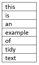

Splitting texts, in our case speeches, into individual words is called tokenization 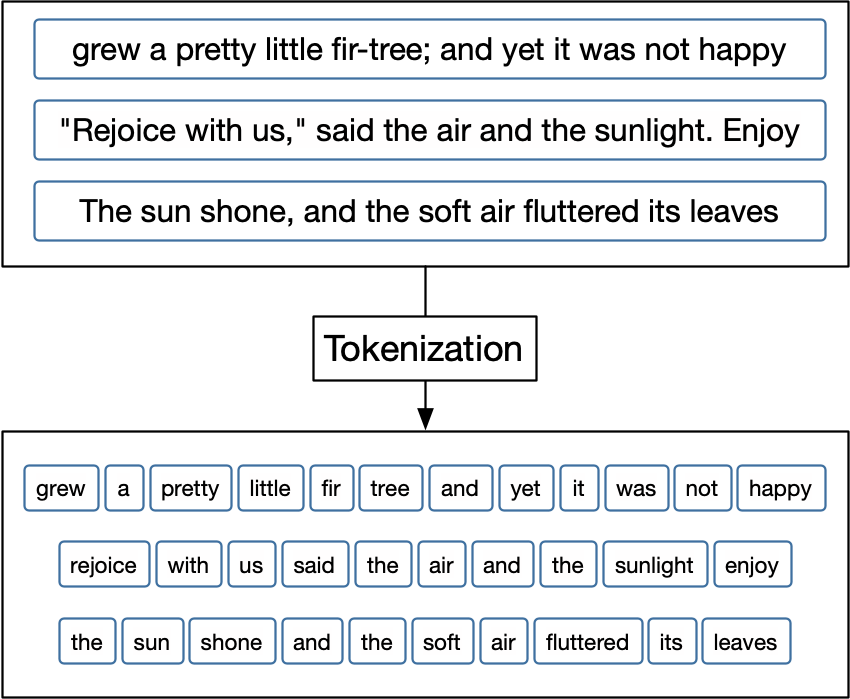Hvitfeldt & Silge, 2021

Tokenization of text into individual words is necessary for text mining because it allows us to analyze the text closely and in detail, analyses which can later be visualized to understand the patterns of the text. Tokenization is language independent, as long as the language is written in an alphabet or syllabary that uses spaces between words. When tokenizing our text to make it tidy, the metadata that describe the whole speech are carried over to also describe the individual word. Thus we can split the text into individual words but still keep track of who said that word and when they did.

We use the tidytext library for tokenization

kina_tidy <- kina %>% 
  unnest_tokens(word, Text) #tidytext tokenization

Stopwords

In all natural language texts, frequent words that carry little meaning by themselves are distributed all across the text

The frequent low-meaning words need to be removed because they do not add anything to our understanding of the texts and are just noise

The tm library contains a list of stopwords for Danish, which we’ll make into a tibble. We have to specify that the list of stopwords that we want to call is the list for the Danish language. Note that stopword lists are also available for most major European languages

stopwords_dansk <- tibble(word = stopwords(kind = "danish"))

Sentiment analysis

Sentiment analysis is a method for measuring the sentiment of a text. To do this, it is necessary to have a list of words that have been assigned to a certain sentiment. This can be a simple assignation of words into positive and negative, it can be an assignation to one among a multitude of categories, and the word can have a value on a scale. In this course we will use the AFINN index for Danish, which assigns approximately 3500 words on a scale from +5 to -5. This will enable us to calculate and compare the overall sentiment of the various speeches. As a side note, AFINN index is also available in English.

We need to download the AFINN Index from GitHub

download.file("https://raw.githubusercontent.com/KUBDatalab/R-textmining/main/data/AFINN_dansk.csv", "data/AFINN_dansk.csv", mode = "wb")

Now we read need to read the AFINN Index into a tibble and rename the columns

AFINN_dansk <- read_csv("data/AFINN_dansk.csv")

Bringing it all together: joins

We have now created tibbles, each with the words appropriate for removal of stopwords and application of sentiment analysis respectively. Now we need to bring them together in the correct order, and we do this by using join-functions. The join functions from the tidyverse library allow tibbles to be joined together based on columns that have cells where the content is the same in both tibbles.

There are fundamentally 2 types of joins:

• Mutating joins (which add columns)
• Filtering joins (which filter away rows)

Mutating joins work by adding new columns to the tibble. We will use left_join, which is the most common of the mutating joins 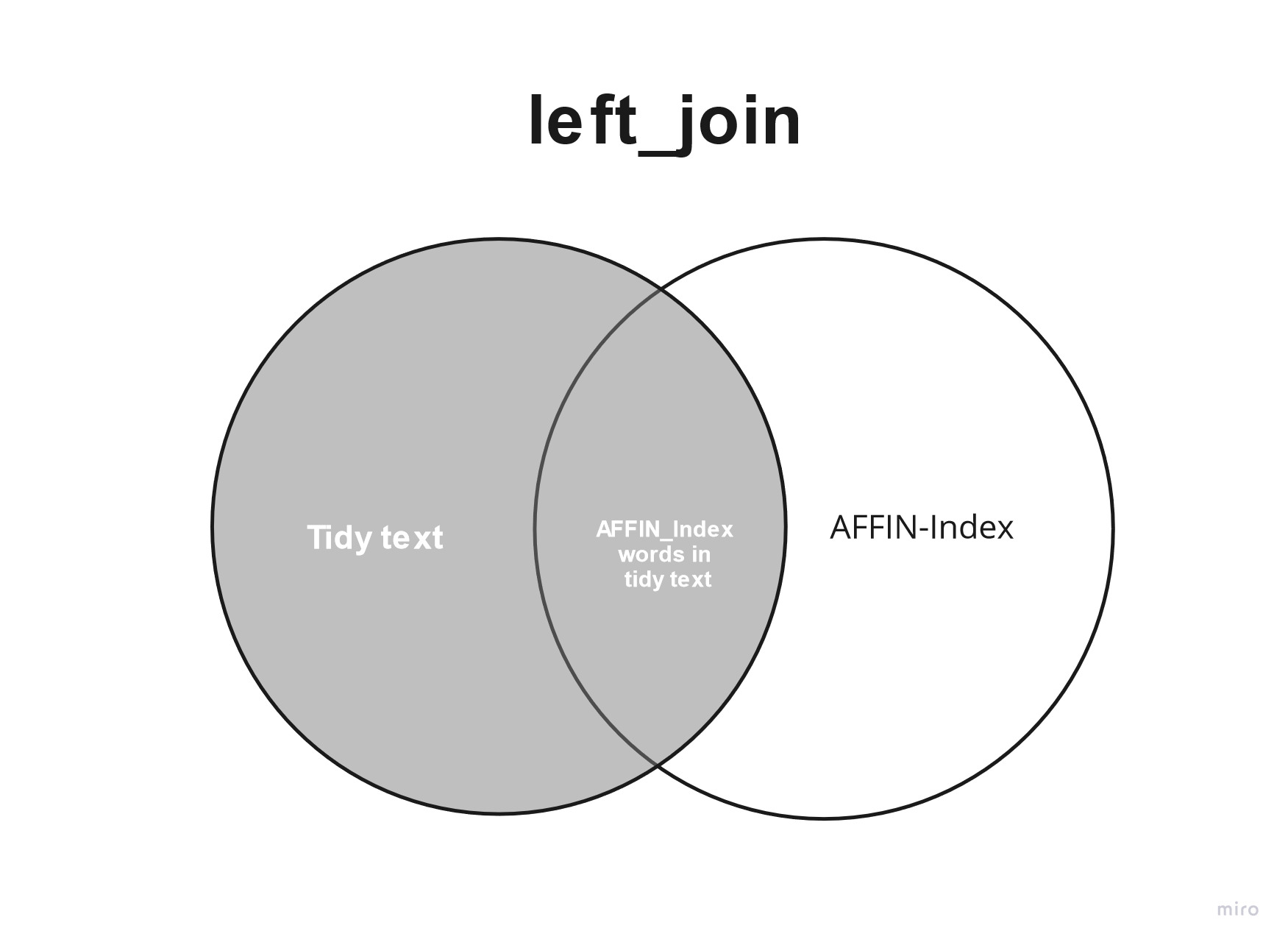The left_join joins all AFINN sentiment values to those rows that contain a word that is in the AFINN Index and adds it as a new column to the tibble. In the new column, the rows that contain words that don’t appear in the AFINN Index have NA in their cell

Filtering joins work by filtering away some rows in the tibble. We will use the anti_join, which removes those rows that contain a word that is also in the stopword list

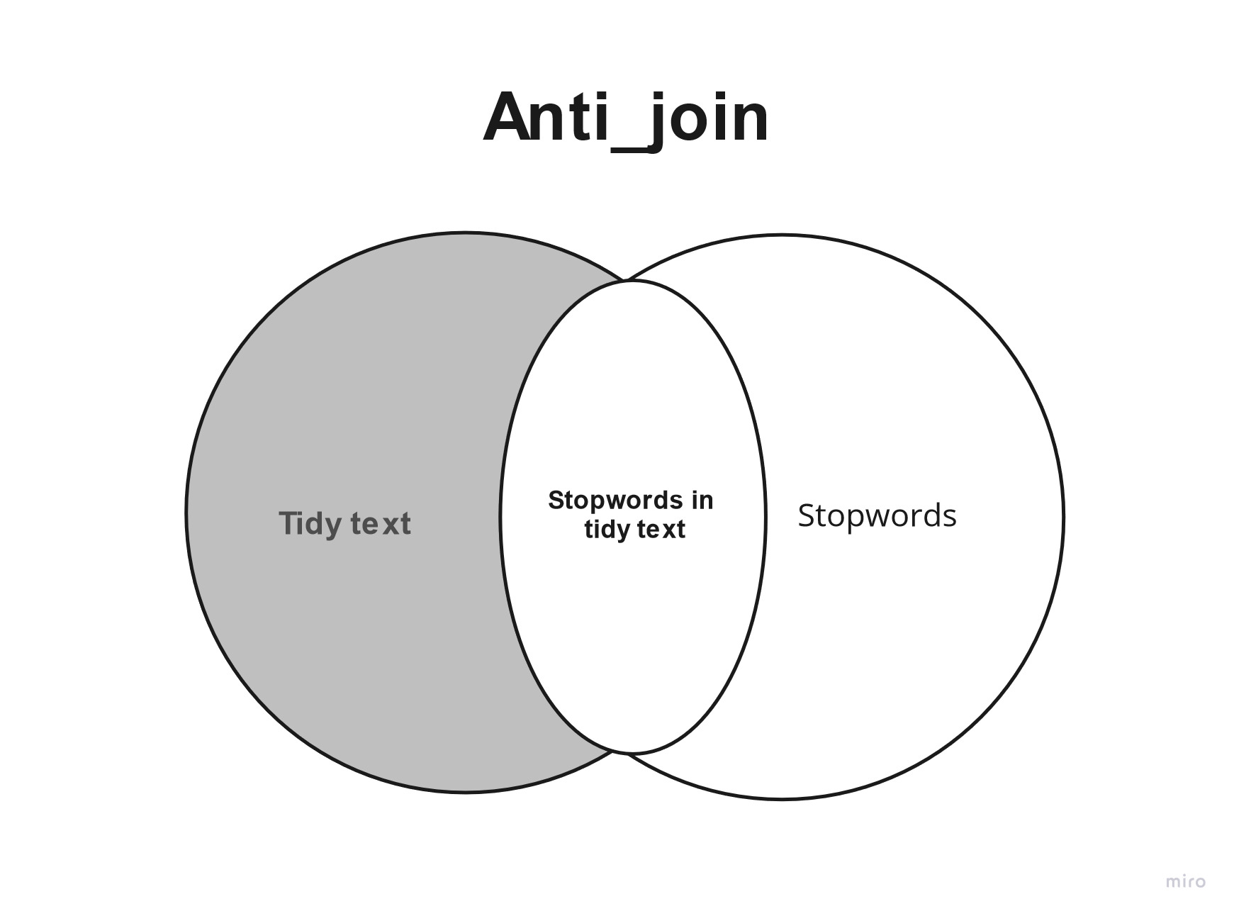
For more info on joins see R for Data Science section section 13: Relational data

We will use the anti_join first, beause we need to filter away stopwords before we analyse the text with sentiment analysis

kina_tidy_2 <- kina_tidy %>% 
  anti_join(stopwords_dansk, by = "word") %>% #stopwords in Danish
  left_join(AFINN_dansk, by = "word") #left join with AFINN Index in Danish

Analyzing the sentiment of parties

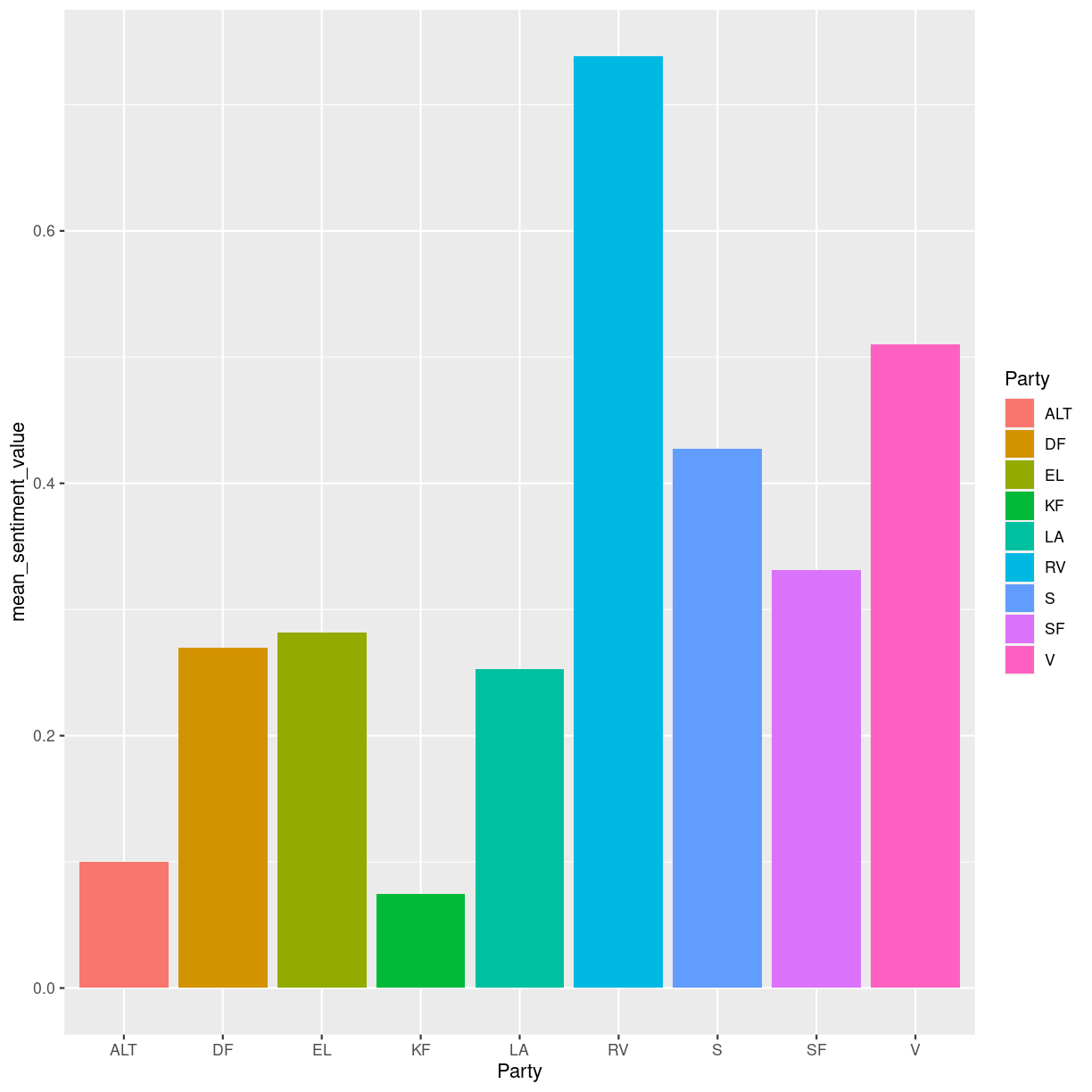
We would like to measure the sentiment of each party when giving speeches on the topic of China

First we need to calculate the mean sentiment value for each party. We save it as an object so that we can easily recall it for visualization

kina_sentiment_value <- kina_tidy_2 %>% 
  filter(Role != "formand") %>% 
  group_by(Party) %>% 
  summarize(
    mean_sentiment_value = mean(sentiment_value, na.rm=TRUE)
  )

Now we want to visualize each party’s mean sentiment value according to the AFINN-Index

kina_sentiment_value %>% 
  ggplot(aes(x = Party, y = mean_sentiment_value, fill = Party)) + 
  geom_col() +
  labs(x= "Party")

Analyzing the sentiment of rød and blå blok

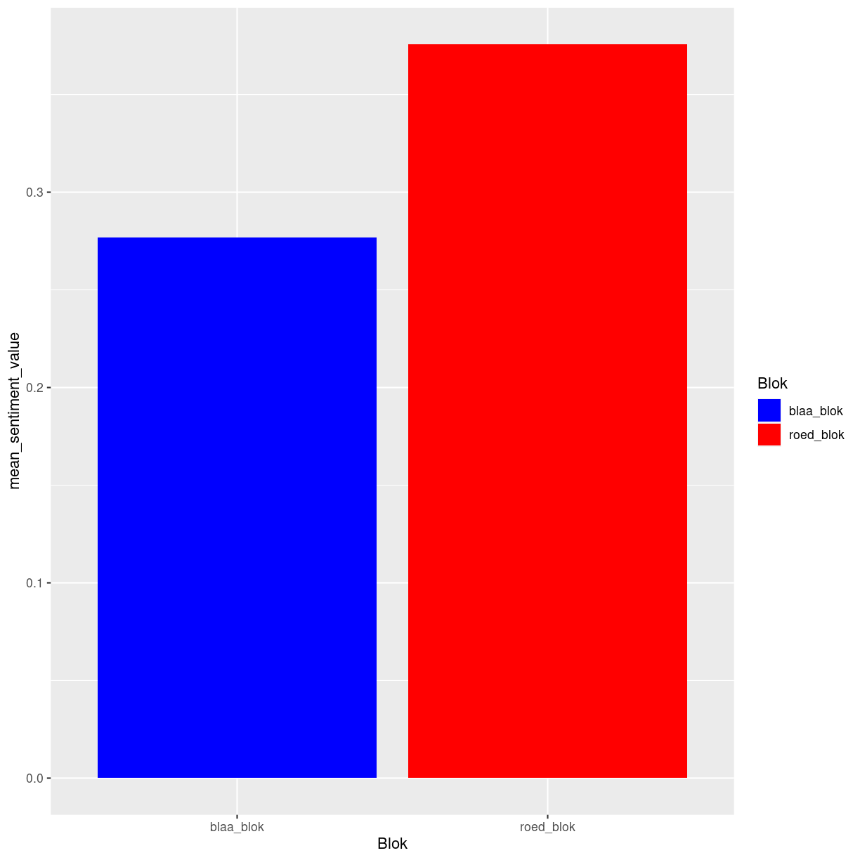
We would also like to analyze the sentiment of rød and blå blok as a whole respectively. To do this, we need to add a column to each row that specifies whether the word comes from a member of a party in rød blok or blå blok. We must therefore first define which parties make up rød and blå blok and put that in a tibble, then bind the two tibbles into one tibble, and then make a left_join to the rows in our tidy text

roed_blok <- tibble(Party = c("ALT", "EL", "SF", "S", "RV"), Blok = c("roed_blok"))
blaa_blok <- tibble(Party = c("V", "KF", "LA", "DF"), Blok = c("blaa_blok"))
blok <- bind_rows(roed_blok, blaa_blok)
kina_tidy_blokke <- kina_sentiment_value %>% 
  left_join(blok, by = "Party")

Now we would like to do the same analysis of mean sentiment value, this time for each blok. We also want to specify that the column for roed_bloek should be red and the column for blaa_blok should be blue

kina_blokke_sentiment_value <- kina_tidy_blokke %>% 
  group_by(Blok) %>% 
  summarize(
    mean_sentiment_value = mean(mean_sentiment_value, na.rm=TRUE)
  )

kina_blokke_sentiment_value %>% 
  ggplot(aes(x = Blok, y = mean_sentiment_value, fill = Blok)) + 
  geom_col() +
  scale_fill_manual(values = c("blue", "red")) +
  labs(x= "Blok")

Key Points

• All natural language texts must be prepared for analysis

Episode 3 word frequency analysis

Overview

Teaching: 0 min
Exercises: 0 min

Questions

• How can we find the most frequent terms from each party?

Objectives

• Learning how to analyze term frequency and visualize it

R Markdown

library(tidyverse)
library(tidytext)
library(tm)

Word frequency

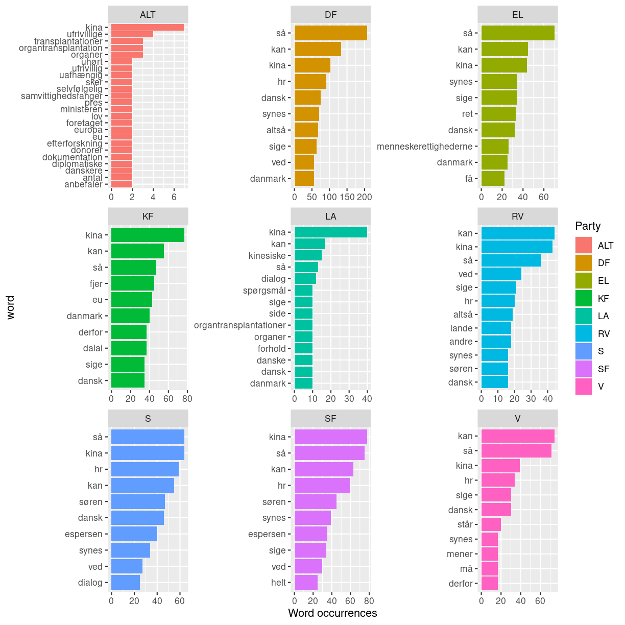
Now that we have seen the average sentiment of the parties, we want to get a deeper understanding of what they talk about when discussing China. We can calculate the most frequent words that each party uses, and then visualize that to get an impression of what they talk about when discussing China.

First we calculate the 10 most frequent words that each party says

kina_top_10_ord <- kina_tidy_blokke %>% 
  filter(Role != "formand") %>% 
  group_by(Party) %>% 
  count(word, sort = TRUE) %>%
  top_n(10) %>% 
  ungroup() %>% 
  mutate(word = reorder_within(word, n, Party))

Selecting by n

Now we want to visualize the result

kina_top_10_ord %>% 
  ggplot(aes(n, word, fill = Party)) +
  geom_col() + 
  facet_wrap(~Party, scales = "free") +
  scale_y_reordered() +
  labs(x = "Word occurrences")

A more extensive stopword list for Danish is the ISO stopword list. We will use it know, so lets download it from the repository. Then we save it as an object. Then we make it into a tibble to prepare it for anti_join with our dataset

download.file("https://raw.githubusercontent.com/KUBDatalab/R-textmining/main/data/iso_stopwords.csv", "data/iso_stopwords.csv", mode = "wb")

iso_stopwords <- read_csv("data/iso_stopwords.csv")

Let us now apply it to the dataset by anti_join

kina_top_10_ord_2 <- kina_tidy_blokke %>% 
  anti_join(iso_stopwords, by = "word")

Unfortunately for us, most of the most common words are words that act like stopwords, carrying no meaning in themselves. To get around this, we can create our own custom list of stopwords as a tibble, and then anti_join it with the dataset, just like we did for the already existing stopword lists.

First we look at the top words to find the stopwords for our custom stopword list. Here I have printed 10, but I have looked at over 70

kina_top_10_ord_2 %>% 
  count(word, sort = TRUE) %>% 
  top_n(10) %>% 
  tbl_df %>% 
  print(n=10)

Selecting by n

# A tibble: 10 × 2
   word           n
   <chr>      <int>
 1 kina         495
 2 hr           476
 3 dansk        278
 4 synes        236
 5 søren        217
 6 ordføreren   197
 7 danmark      193
 8 tak          189
 9 espersen     175
10 altså        160

Based on this, we select the words that we consider stopwords and make them into a tibble. We also want to include among our stopwords the word Danmark and its genitive case and derivative adjectives, because Denmark of course is frequently named in a Danish parliamentary debate and adds little to our analysis and understanding. Let’s also remove the name China, its genitive case and derivative adjectives, because we know that the debate is about China. Let’s also remove words that state the title or role of a member of the parliament. Let’s also remove the words spørgsmål and møder, as it relates internal questions and meetings among the members of parliament. Let’s also remove the words about Folketingets Præsidium, which do not pertain to the content of the debate. Upon later examinations some more names have also been added to the custom stopword list

custom_stopwords <- tibble(word = c("så", "kan", "hr", "sige", "synes", "ved", "altså", "søren", "tror", 
                                    "få", "bare", "derfor", "godt", "andre", "må", "espersen", "mener", "gøre", "helt", "dag", 
                                    "faktisk", "folkeparti", "gerne", "side", "gør", "nogen", "fordi", "hvordan", "tak",
                                    "måde", "set", "siger", "andet", "sagt", "år", "lige", "står", "tage", "nemlig", "lidt",
                                    "sag", "går", "kommer", "nok", "danmark", "danmarks", "dansk", "danske", "danskt", 
                                    "kina", "kinas", "kinesisk", "kinesiske", "kinesiskt", "kineser", "kineseren", 
                                    "kinesere", "kineserne", "ordfører", "ordføreren", "ordførerens", "ordførere", "ordførerne", 
                                    "spørgsmål", "møder", "holger", "k", "nielsen", "regering", "regeringen", "regeringens", 
                                    "folketinget", "folketingets", "måske", "forslag", "egentlig", "rigtig", "rigtigt", "rigtige", 
                                    "hvert", "bør", "grund", "vigtig", "vigtigt", "vigtige", "ting", "ønsker", "fru", "hr", 
                                    "selvfølgelig", "gange", "præcis", "sagde", "hele", "fald", "enhedslisten", "sidste", 
                                    "forstå", "betyder", "alliances", "fortsat", "venstre", "holde", "præsidium", "baseret",
                                    "lande", "land", "gjorde", "pind", "simpelt", "frem", "præsidiet", "præsidium", 
                                    "dokument", "tale", "hen", "o.k", "alverden", "angiveligt"))

We then do an anti_join of our custom stopword list to our tidy text

kina_top_10_ord_3 <- kina_top_10_ord_2 %>% 
  anti_join(custom_stopwords, by = "word")

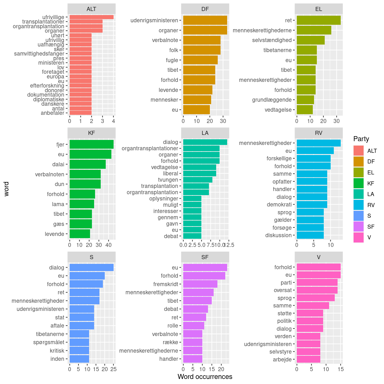
Let’s now calculate the top 10 words from each party and save it as an object

kina_top_10_ord_4 <- kina_top_10_ord_3 %>% 
  filter(Role != "formand") %>% 
  group_by(Party) %>% 
  count(word, sort = TRUE) %>%
  top_n(10) %>% 
  ungroup() %>% 
  mutate(word = reorder_within(word, n, Party))

Selecting by n

Let us now plot the result

kina_top_10_ord_4 %>% 
  ggplot(aes(n, word, fill = Party)) +
  geom_col() + 
  facet_wrap(~Party, scales = "free") +
  scale_y_reordered() +
  labs(x = "Word occurrences")

tf_idf

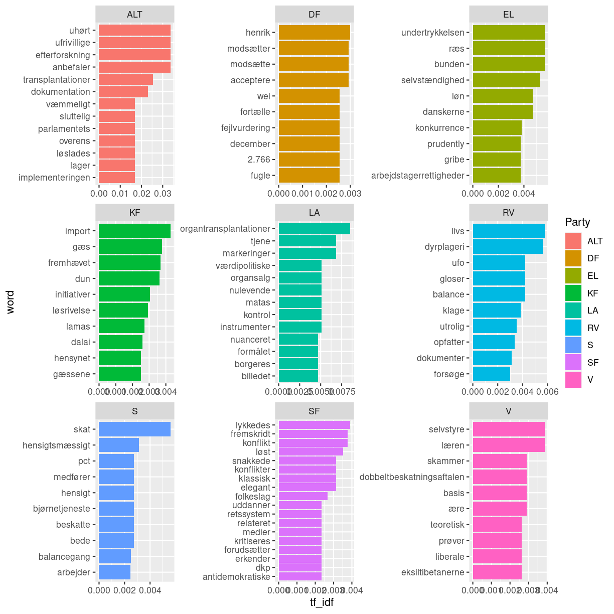
We see that many words co-occur among the parties. How can we make a plot of what each party talks about that the others don’t? We can use the tf_idf calculation. Briefly, tf_idf in this case looks at the words that occur among each party, and gives a high value to those that frequently occur in one party but rarely occur among the other parties. This will give us a sense of what each party emphasizes in their speeches about China

First we need to calculate the tf_idf of each word in our tidy text

kina_tidy_tf_idf <- kina_top_10_ord_3 %>% 
  filter(Role != "formand") %>% 
  count(Party, word, sort = TRUE) %>% 
  bind_tf_idf(word, Party, n) %>% 
  arrange(desc(tf_idf))

Now we want to select each party’s 10 words that have the highest tf_idf

kina_tidy_tf_idf_top_10 <- kina_tidy_tf_idf %>% 
  group_by(Party) %>% 
  top_n(10) %>% 
  ungroup() %>% 
  mutate(word = reorder_within(word, tf_idf, Party))

Selecting by tf_idf

Now let’s make our plot.

kina_tidy_tf_idf_top_10 %>%  
  ggplot(aes(tf_idf, word, fill = Party)) +
  geom_col() +
  facet_wrap(~Party, scales = "free") +
  scale_y_reordered() +
  labs(x = "tf_idf")

Key Points

• Custom stopword list may be necessary depending on the context

Episode 4 text mining extras

Overview

Teaching: 0 min
Exercises: 0 min

Questions

• More resources

Objectives

• Learning about extra tools that can aid your text mining journey

Stopwords for other languages

Stopword lists are available for a range of European languages via the tm library. See documentation on https://cran.r-project.org/web/packages/tm/tm.pdf p. 38

To call the stopword list for a certain language and make it a tibble to easily anti_join with your tidy text run the following code and insert the name of the language if a stopword list exists for it

stopwords_your_chosen_language <- as_tibble(stopwords(kind = "yourchosenlanguage"))

Stemming as Natural Language Processing

One data preparation technology that we didn’t use in this course is stemming. Stemming takes the inflectional morphological endings typically found at the end of words in Indo-European and Uralic languages and removes them, so that you don’t need to put all potential morphological endings in a stopword list to catch all instances of a word. This is especially useful in languages with lots of verb conjugations and noun declensions like the Romance languages and the Slavic languages. BE AWARE that many Danish and English sentiment indexes don’t work on stemmed words but take the limited morphological variation in these languages into account. As a rule of thumb, if you want to do sentiment analysis for a Danish or English text, then you are best of with not using stemming

It is possible to stem in a variety of European languages using the Porter-stemmer via the library SnowballC. Start by getting of list of which languages the stemmer can handle

install.packages("SnowballC")
library(SnowballC)
getStemLanguages()

Use stemming on the column with text in your tibble

tibble$stemmed_text <- wordStem(tibble$column_with_text, language = "name of the language")

How to download the full dataset

Go to https://repository.clarin.dk/repository/xmlui/handle/20.500.12115/44 and click the blue button that says: Download all files in item. This will download all approximately 860 files in Zip folder. The Zip folder contains zip folders for each year in the dataset, and these zip folders contain the parliament speeches including the metadata that describe them as .txt files. You need to create a new folder somewhere outside the zip folder environment. Now you must copy-paste all .txt files to that new folder. You can go into each zip-folder, press Ctrl+a to mark all files, and then press Ctrl+c to copy them. Go to the new folder and press Ctrl+v

To import the files into R as one tibble, you must first set the working directory to your new folder. Then run the following code:

files <- dir(pattern = "*.txt")

data <- files %>% 
  map(read_delim) %>% 
  reduce(rbind)

This may take up to 10 minutes. Once you have read all the files in as one tibble, you want to make it into one new file, so that you can quickly load the whole dataset in next time. Run the following code to write the file but insert the place on the C drive via the tabulator-function and finish the string with the name of your new file and put .txt after the filename:

write_delim(data, "C:/Users/yourusername/Desktop/Folder/Folketinget/filename.txt")

Now you can quickly load it in next time by using read_delim. Use filter to filter your dataset however you like it. For more info on the filter function, see https://r4ds.had.co.nz/transform.html section 2

Reading other types of files

You can also use read_csv to read .csv files in the same manner that you read .txt files

Recommended materials

I highly recommend the book Text Mining with R: A Tidy Approach, which is openly available at https://www.tidytextmining.com/ There you can learn more advanced analyses as well as see the application of this course’s methods to different datasets

References

Hvitfeldt, E., & Silge, J. (2021). Supervised Machine Learning for Text Analysis in R (1st ed.). Chapman and Hall/CRC. https://doi.org/10.1201/9781003093459

David Robinson, & Julia Silge. (2017). Text Mining with R. O’Reilly Media, Inc.

Key Points

• Stemming can be useful for Natural Language Processing; Stopword lists are available for many languages