Distributions

Overview

Teaching: 0 min
Exercises: 0 min

Questions

• What are histograms?

• What are violin plots?

• What are density plots?

• What are boxplots?

Objectives

• FIXME

We have some data on the mass of penguins. We expect some penguins to weigh more than others. Perhaps it is a smaller kind of penguin. Perhaps it is a female penguin, and they are smaller than male penguins. And maybe some penguins are fatter than other penguins.

Ranking penguins from light to heavy, how many are there at each weight, or, what is the distribution of their weight?

The plots in this section are useful for visualizing distributions of data.

Histograms

What are they?

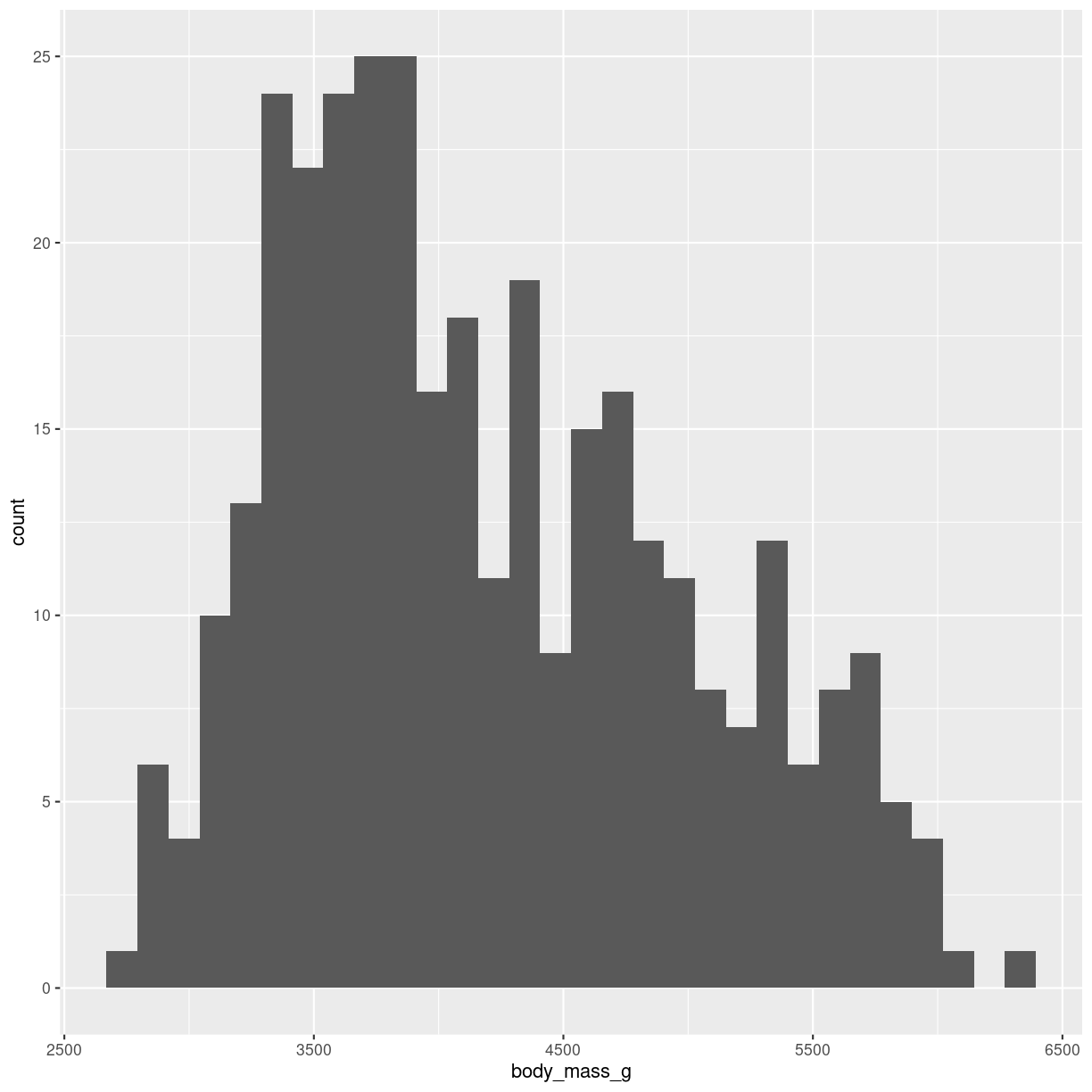
Histograms takes all the weights of the penguins, divides them into intervals, or bins, of weight, eg one bin with 3300 to 3400 grams, and the next bin from 3400 to 3500 grams. Then we count how many penguins are in a specific bin. And plot it. It might look like this:

plot of chunk histogram-show

What do we use them for?

We typically use histograms to visualise the distribution of a variable. Is it normal, bimodal, uniform or skewed? It can quickly reveal mistakes in data or weird outliers.

We can also use histograms to compare different variables. But beware of comparing too many, it can make the graphs difficult to read, and the aim of visualising is to make things easier to understand.

How do we make them?

The geom_ we are using here is geom_histogram(). It takes only one variable in the mapping.

ggplot(penguins, aes(x=body_mass_g)) + 
  geom_histogram()

`stat_bin()` using `bins = 30`. Pick better value with `binwidth`.

plot of chunk histogram-making

Built into the geom_histogram is the statistical transformation, that counts the number of observations in each bin.

Note the message that this statistical transformation as default uses bins = 30. This is the default number of bins. And it is almost guaranteed that it is not the best number of bins.

Bins can be determined in two ways, either by providing a number of bins:

geom_histogram(bins = 30)

or by specifying the width of the bins:

geom_histogram(binwidth = 500)

Interesting variations

More than one distribution on same axis

We can plot more than one distribution in the same plot.

The addition of alpha = 0.6 makes the bars transparent.

penguins %>%
  filter(!is.na(sex)) %>% 
  ggplot( aes(x=body_mass_g, fill=sex)) +
  geom_histogram(alpha = 0.6)

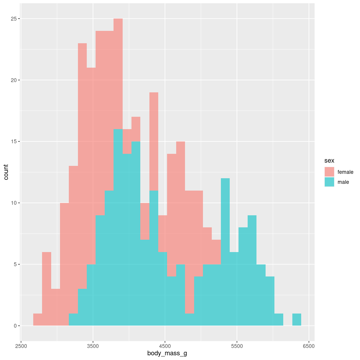
plot of chunk unnamed-chunk-2

We do not map sex to color, but rather to fill. Color is the color of the outline of the individual bars, fill the inside of the bars.

Upside-down

Or mirrored histogram. One distribution above the x-axis, one below.

The code gets a bit more readable if we construct two different dataframes, one for each sex. The statistical transformation that counts the observations in each bin was build into geom_histogram. We now need to plot the negative count for one of the dataframes. Therefore we have to specify the statistical transformation, in order to place a minus sign in front of it in the second line.

Two individual dataframes are plotted, and we have to specify color, since there is no grouping variabel that can be mapped to the fill argument:

male <- penguins %>% 
  filter(sex == "male")
female <- penguins %>% 
  filter(sex == "female")
ggplot() +
  geom_histogram(aes(x = female$body_mass_g), fill="#69b3a2" ) +
  geom_histogram(aes(x = male$body_mass_g, y = -..count.. ), fill= "#404080")

Warning: The dot-dot notation (`..count..`) was deprecated in ggplot2 3.4.0.
ℹ Please use `after_stat(count)` instead.
This warning is displayed once every 8 hours.
Call `lifecycle::last_lifecycle_warnings()` to see where this warning was
generated.

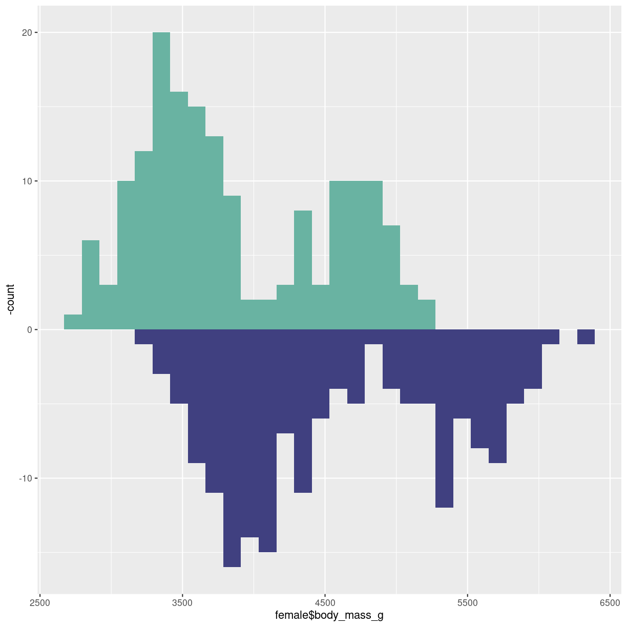
plot of chunk histogram-mirror

Grid

Trying to plot more than two, max three distributions in the same histogram is bad pratice because it becomes difficult to visually separate the different distributions A good workaround is to plot small multiples.

We use facetwrap:

penguins %>% 
  filter(!is.na(sex)) %>% 
  ggplot(aes(body_mass_g)) +
  geom_histogram() +
  facet_wrap(vars(species), nrow = 2)

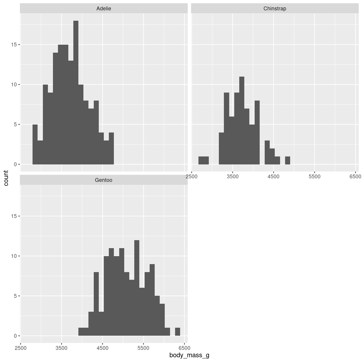
plot of chunk histogram-grid

Rather than specifying the variable used to split the data using vars(species), it can be specified using the formula notation ~species.

nrows and ncols specify the number of rows and columns respectively the the grid.

We can facet wrap on more that one variable:

penguins %>% 
  filter(!is.na(sex)) %>% 
  ggplot(aes(body_mass_g)) +
  geom_histogram() +
  facet_wrap(vars(sex, species))

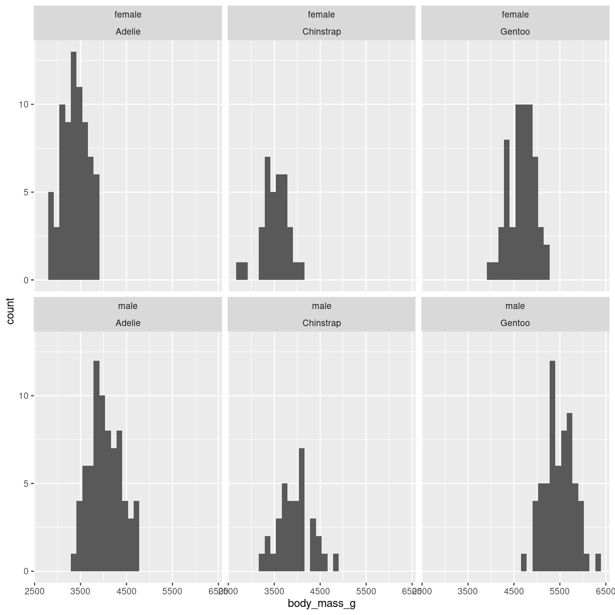
plot of chunk histogram-grid-2

It is also possible to place the six plots in a grid. In that case we use the facet_grid() function:

penguins %>% 
  filter(!is.na(sex)) %>% 
  ggplot(aes(body_mass_g)) +
  geom_histogram() +
  facet_grid(rows = vars(sex), cols= vars(species))

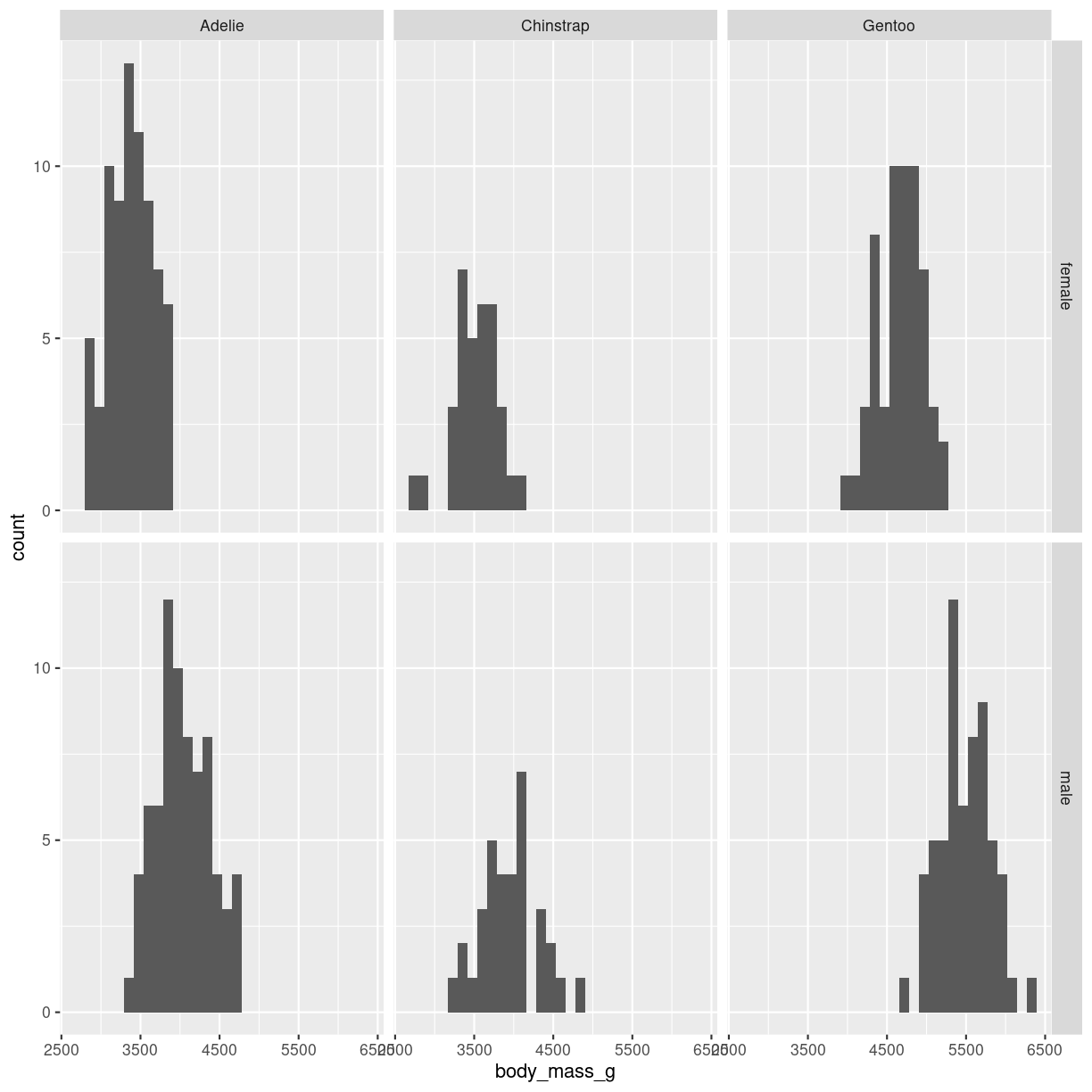
plot of chunk histogram-grid-3

This provides a more consistent presentation of the two facets.

Facetting on more than two variable can get confusing, but can be done.

Think about

The number of bins (or their width, these two are equivalent) can lead to very different conclusions. Try several sizes.

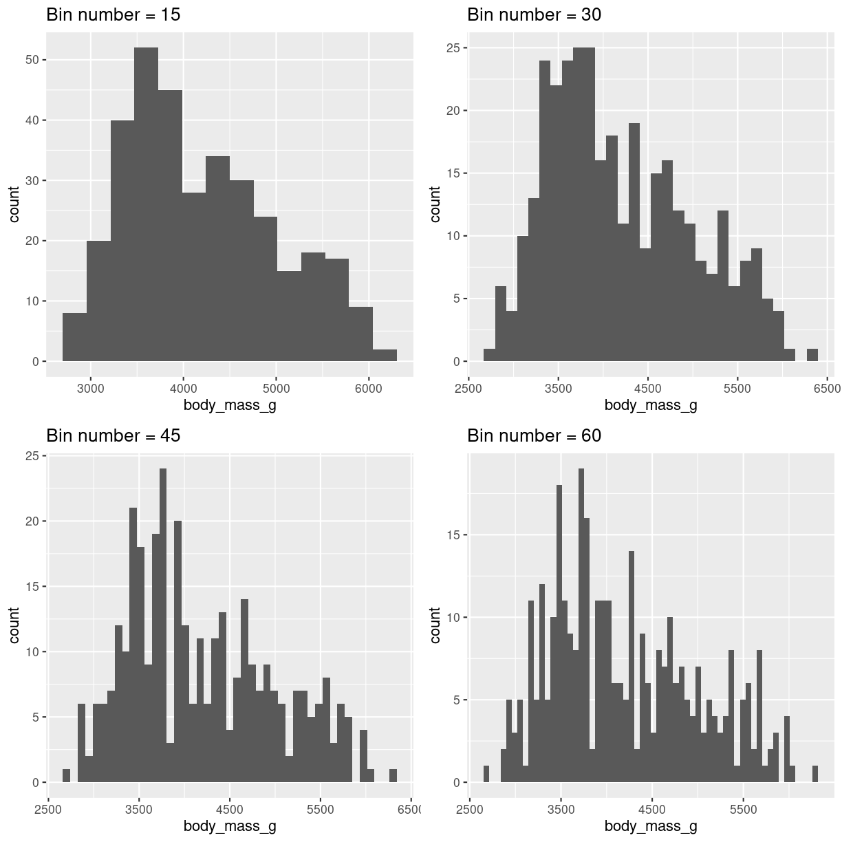
plot of chunk histogram-bin-choices

• Weird and complicated color schemes does not add insight. Avoid them.
• This is not a barplot! Histograms plot the distribution of a single variable.
• Avoid comparing more than two, maybe three groups in the same histogram.
• Do not use unequal bin widths.

Boxplots

What are they?

A summary of one numeric variable. It has several elements.

• The line dividing the box represents the median of the data.
• The ends of the box represents the upper and lower quartiles, (Q3 and Q1 respectively). 50% of the observations are in this box. This is also called the interquartile range (IQR).
• The line at the top of the box, shows Q3 + 1.5 * IQR. This is interpreted as the values above Q3 that are not outliers.
• The line at the bottom of the box, shows Q1 + 1.5 * IQR. This is interpreted as the values below Q1 that are not outliers.
• Dots at each end of the lines shows potential outliers.

plot of chunk boxplot-what

What do we use them for?

A boxplot summarises several important numbers related to the distribution of data. A rule of thumb (but not necessarily a good one), is that if two sets of data do not have overlapping boxes, they come for different distributions, and are therefore different. Typically we show more than one boxplot, but a collection of boxplots.

how do we make them?

penguins %>% 
  ggplot(aes(x = body_mass_g)) + 
  geom_boxplot()

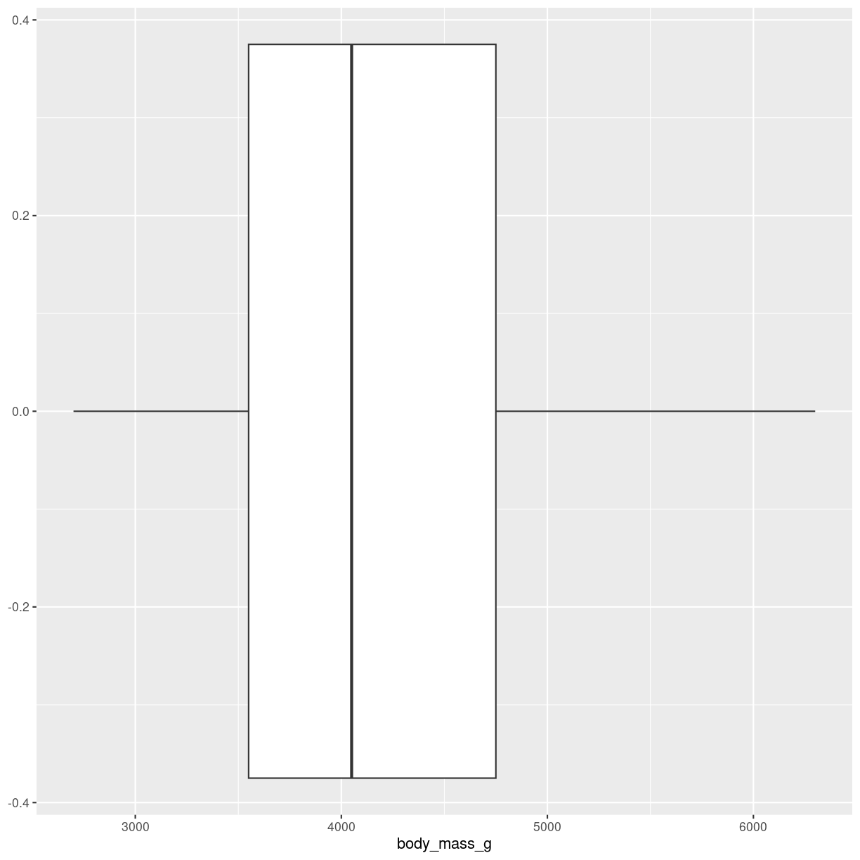
plot of chunk boxplot-how

Typically we want to compare the weight of different groups of penguins. That is, compare the distribution of something, between different groups:

penguins %>% 
  ggplot(aes(y = species, x = body_mass_g)) + 
  geom_boxplot()

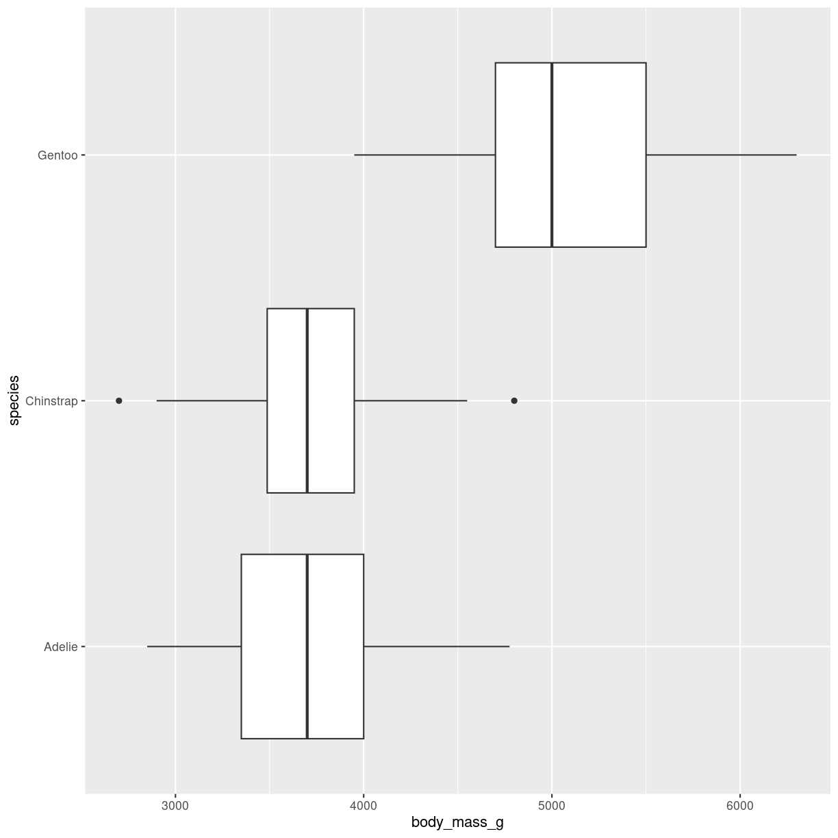
plot of chunk boxplot-groups

Interesting variations

Boxplot with datapoints

geom_jitter adds small amounts of noise to the points. Points can also be added using geom_point()

penguins %>% 
  ggplot(aes(y = species, x = body_mass_g)) + 
  geom_boxplot() +
  geom_jitter()

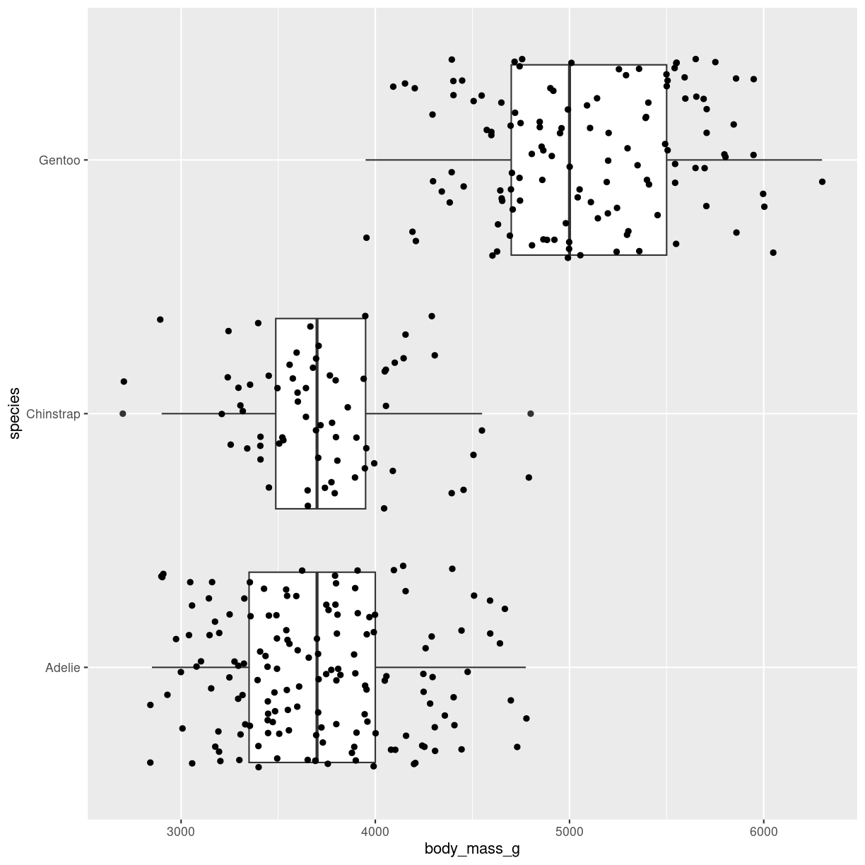
plot of chunk boxplot_jitter

Notches and coloring outliers

penguins %>% 
  ggplot(aes(y = species, x = body_mass_g)) + 
  geom_boxplot(
    notch = T,
    notchwidth = 0.5,
    outlier.color = "red"
  )

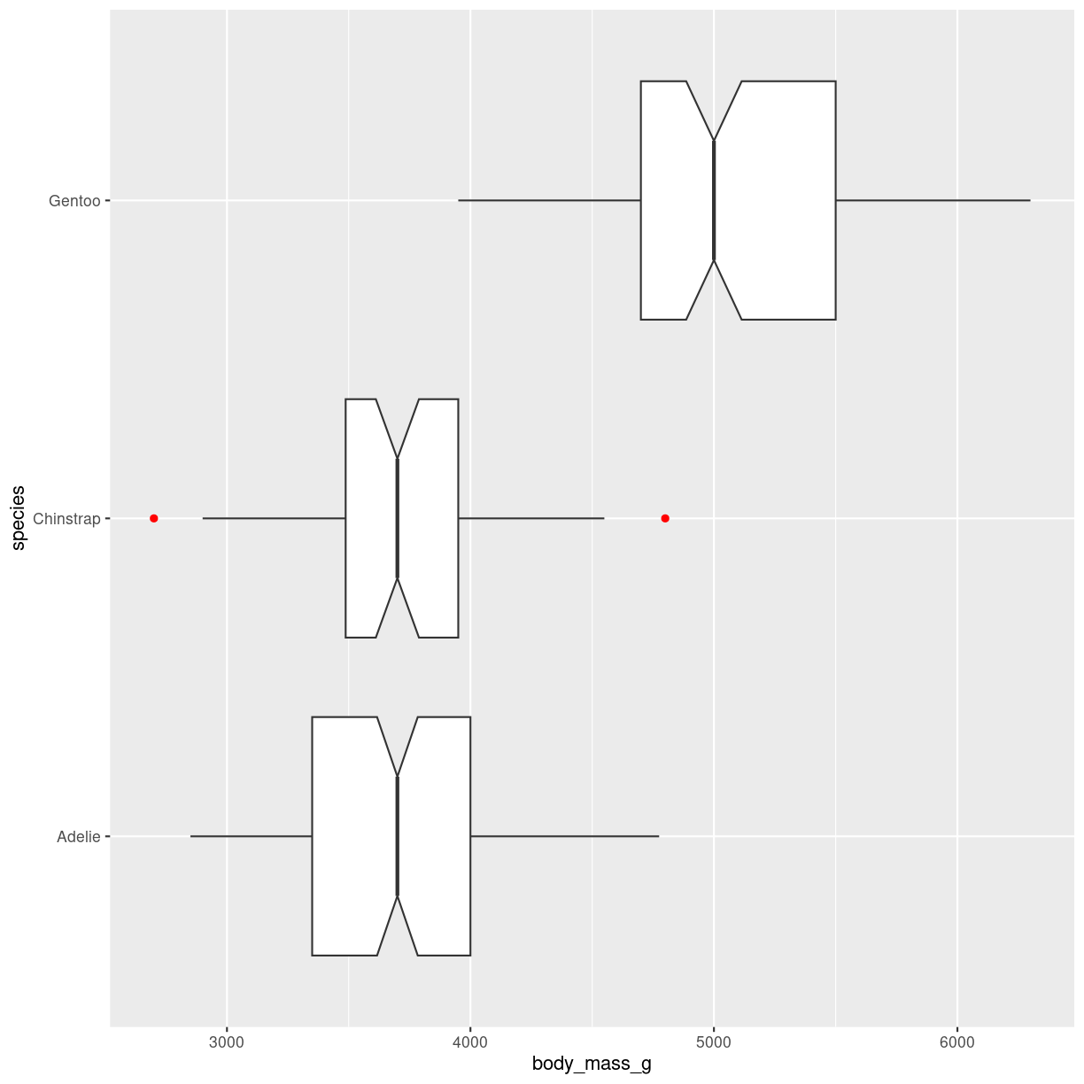
plot of chunk notched-box

Outlier shape, fill, size, alpha and stroke can be controlled in similar ways.

Variable width of boxes

varwidth = T will adjust the width of the boxes proportional to the squareroot of the number of observations in the groups.

penguins %>% 
  ggplot(aes(y = species, x = body_mass_g)) + 
  geom_boxplot(
   varwidth = T
  )

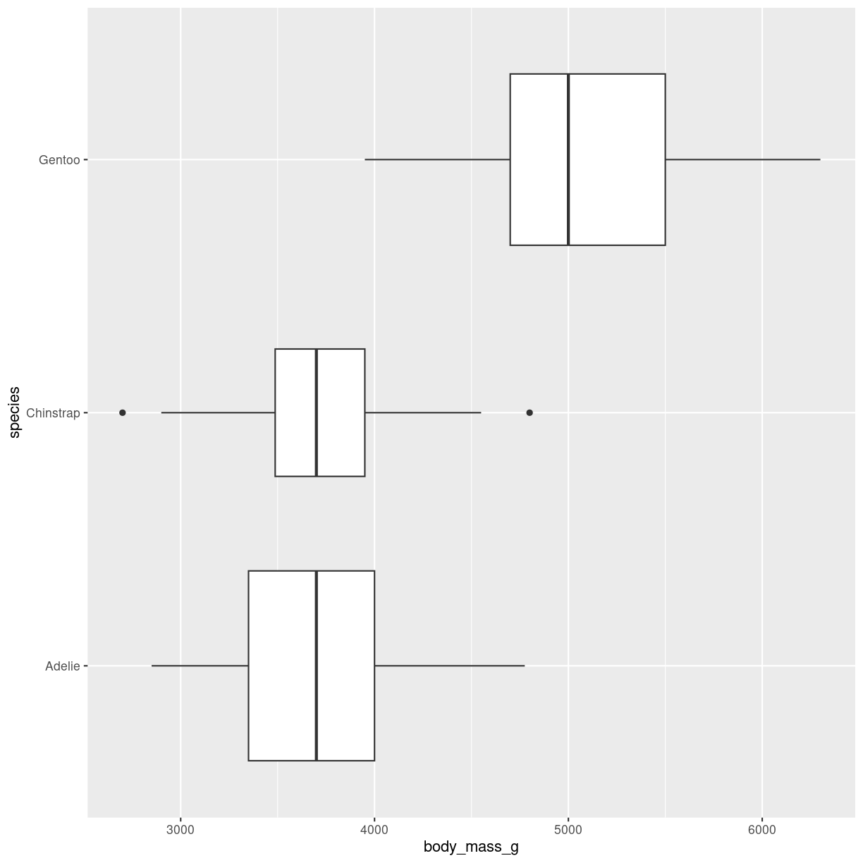
plot of chunk boxplot-var-width

Think about

Boxplots might hide features of the data. The two plots below show first two boxplots that are made from different distributions. The overlap might lead us to think they are similar. The plot on the right adds the individual datapoints revealing that the data is not that similar.

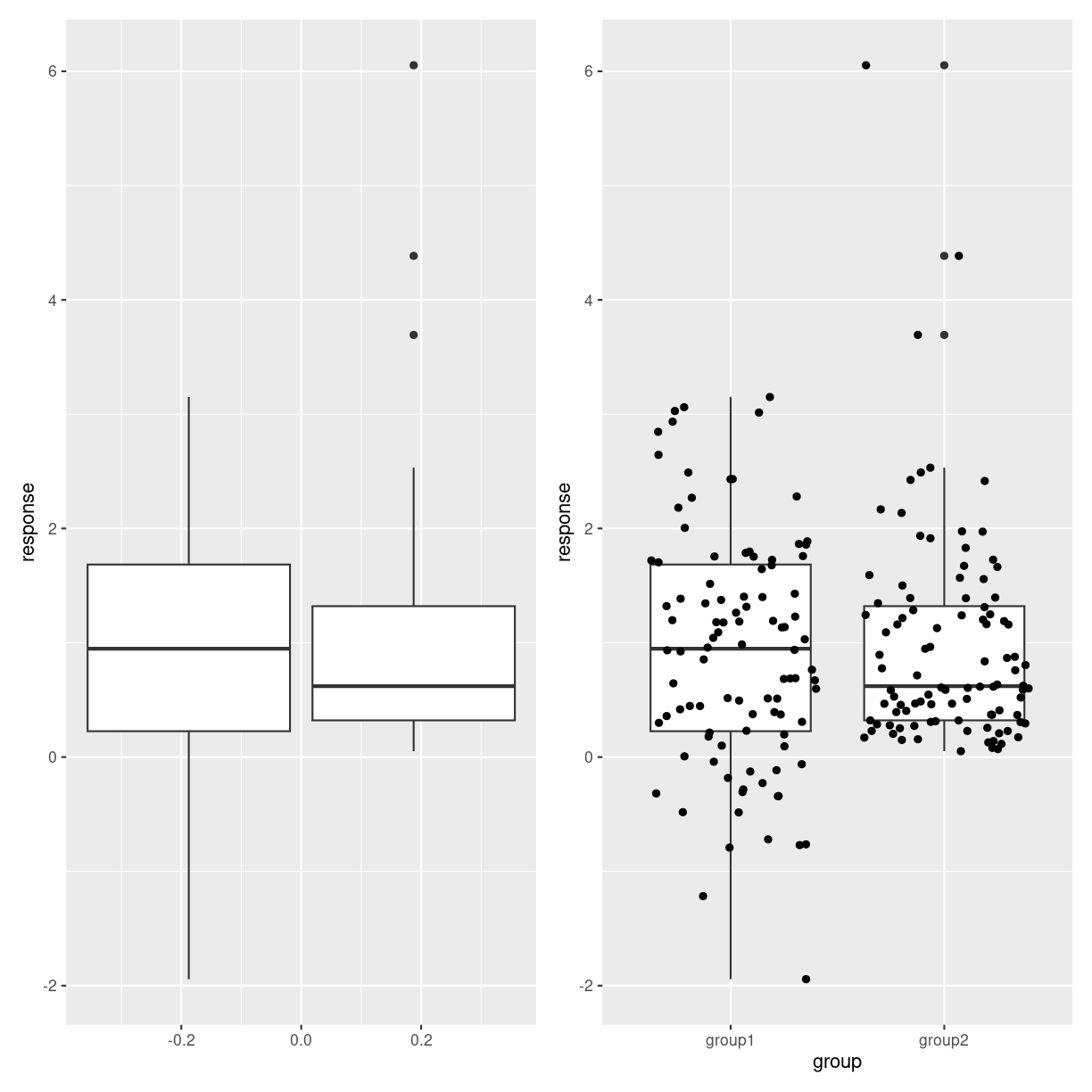
plot of chunk boxes_hiding_stuff

Density plots

What are they?

A plot of the kernel density estimation of the distribution.

Think of it as a smoothed histogram.

`stat_bin()` using `bins = 30`. Pick better value with `binwidth`.

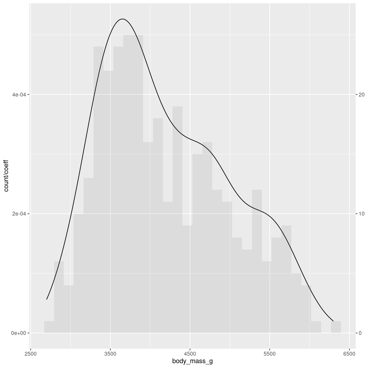
plot of chunk density-what

What do we use them for?

Density plots show the distribution of a numeric variabel. It gets a bit closer to an actual continuous distribution than a histogram.

How do we make them?

As with histograms we only use one variable:

penguins %>% 
  ggplot(aes(body_mass_g)) + 
  geom_density() 

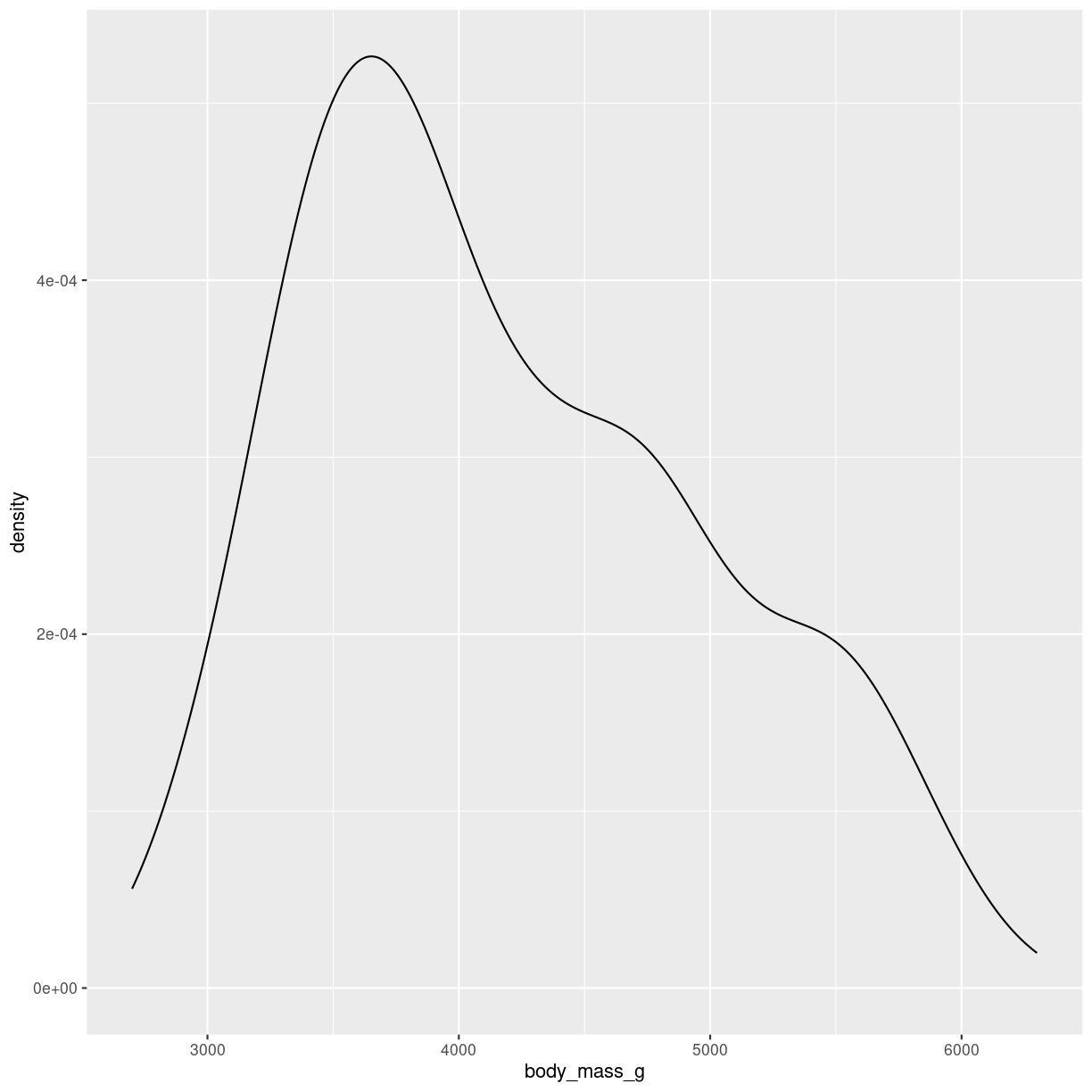
plot of chunk density-how

Interesting variations

More than one distribution on same axis

Upside-down

Made in almost the same way as the mirrored histogram:

male <- penguins %>% 
  filter(sex == "male")
female <- penguins %>% 
  filter(sex == "female")
ggplot() +
  geom_density(aes(x = female$body_mass_g), fill="#69b3a2" ) +
  geom_density(aes(x = male$body_mass_g, y = -..density.. ), fill= "#404080")

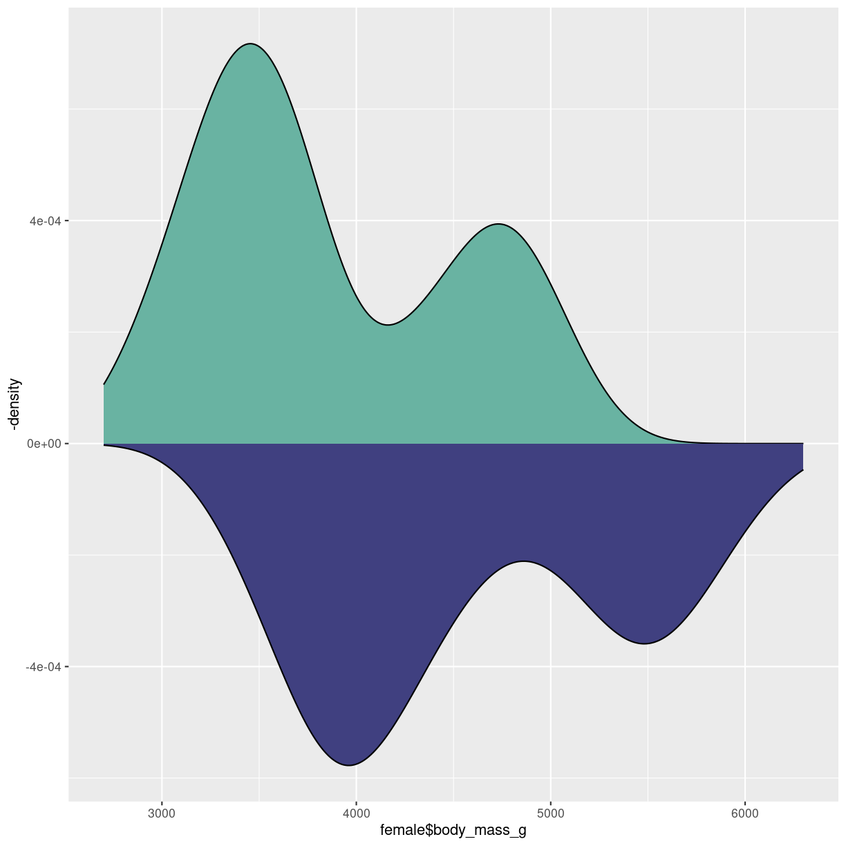
plot of chunk density-mirror

Grid

Fuldstændigt parallelt til grids i histogrammer

Think about

Ridgeline

library(ggridges)

What are they?

Det kan se ret cool ud. Det er grundlæggende “bare” et sæt af flere densityplots.

Også kendt som joyplots

Ren

Loading required package: viridisLite

Picking joint bandwidth of 153

Warning: Removed 2 rows containing non-finite values (`stat_density_ridges()`).

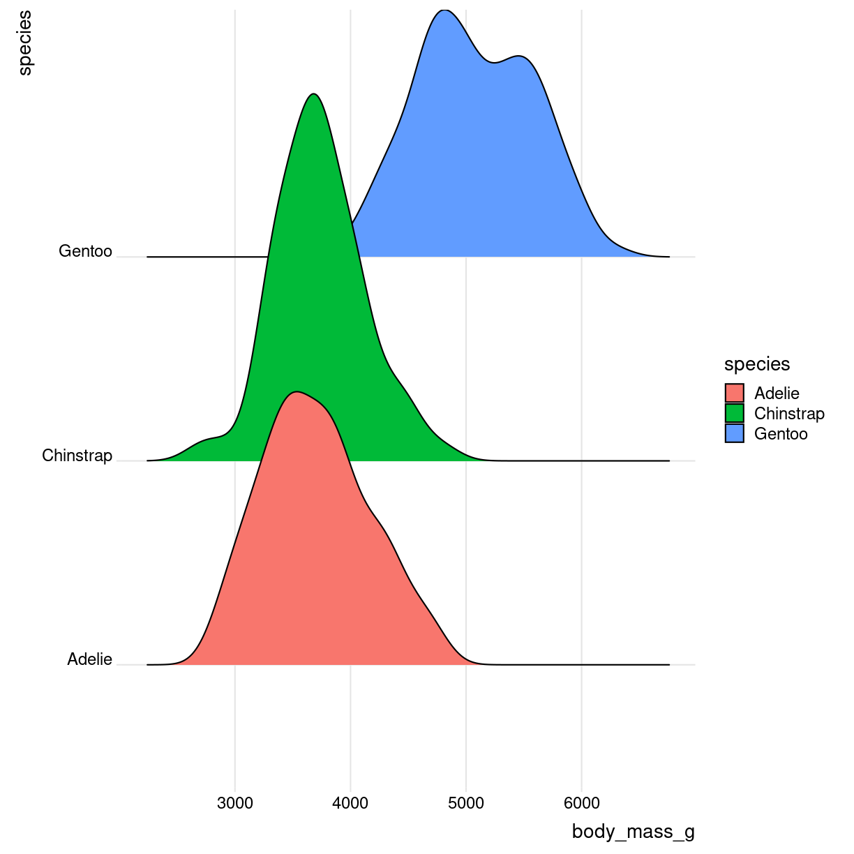
plot of chunk ridges-what

What do we use them for?

how do we make them?

library(ggridges)

penguins %>% 
  ggplot(aes(x = body_mass_g, y = species, fill = species)) +
  geom_density_ridges()  +
    theme_ridges() 

Picking joint bandwidth of 153

Warning: Removed 2 rows containing non-finite values (`stat_density_ridges()`).

plot of chunk ridges-how

Interesting variations

Og med farvelægning efter vægt

library(ggridges)
library(viridis)
penguins %>% 
  mutate(body_mass_g = as.numeric(body_mass_g)) %>% 
  ggplot(aes(x = body_mass_g, y = species, fill = ..x..)) +
  geom_density_ridges_gradient()  +
    theme_ridges() 

Picking joint bandwidth of 153

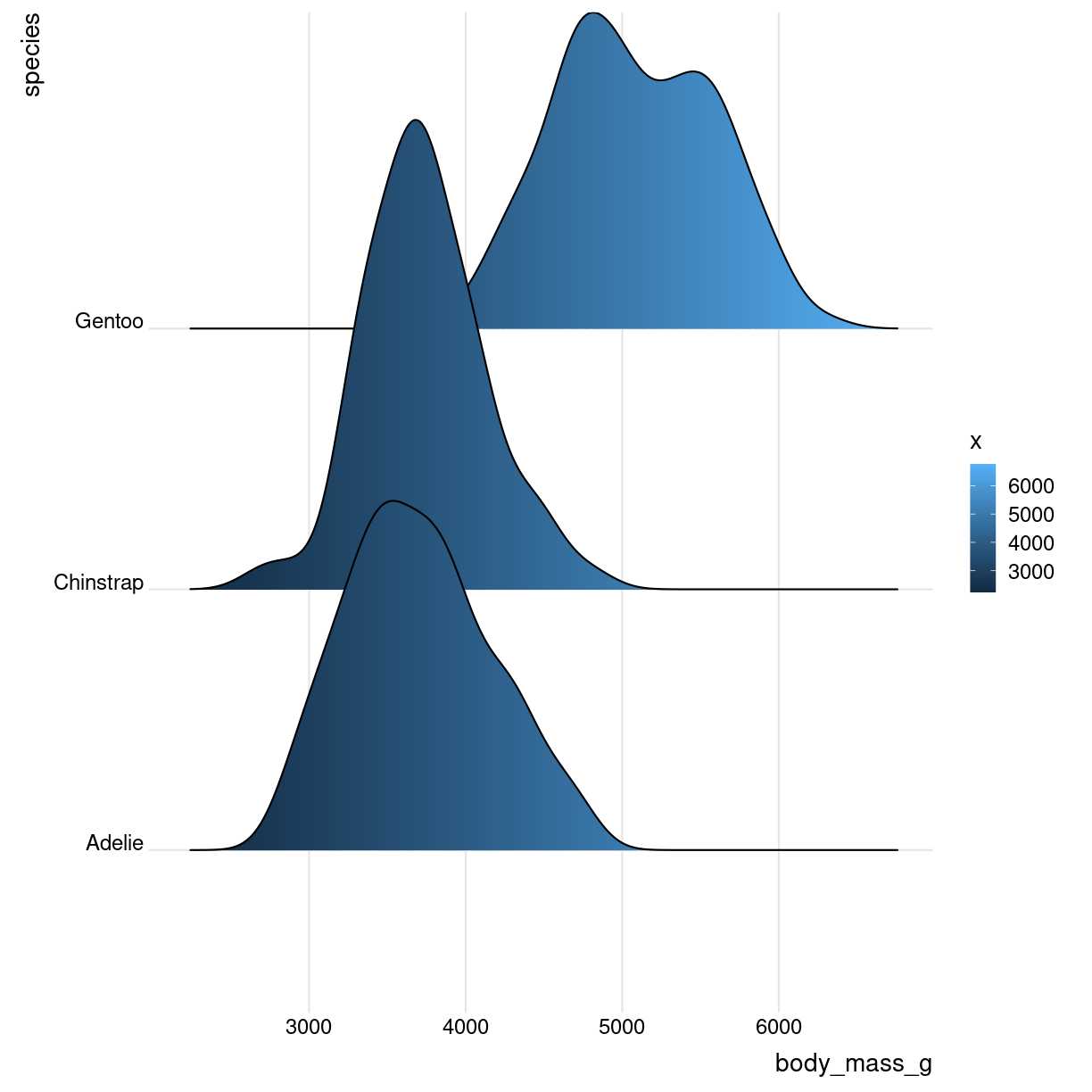
plot of chunk unnamed-chunk-4

Think about

Violin

What are they?

en slags boxplot. formen repræsenterer density. På mange måder bedre end boxplots. Men stiller lidt større krav til folk der har vænnet sig til at læse boxplots.

penguins %>% 
  ggplot(aes(body_mass_g, y = species, fill = species)) +
  geom_violin() +
  coord_flip()

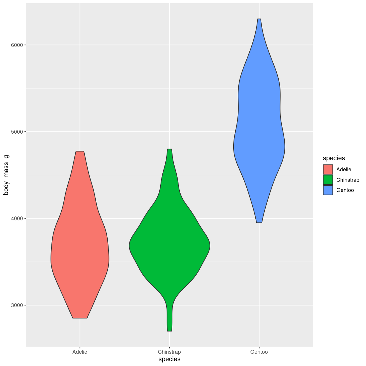
plot of chunk violin-what

What do we use them for?

Tillader os både at se en ranking af forskellige grupper - og deres fordelinger.

how do we make them?

geom_violin()

Interesting variations

Think about

Pas på med at bruge dem hvis datasæt er for små. Da vil et boxplot med jitter ofte være bedre.

sorter/order grupperne efter median-værdien.

Hvis der er meget forskellige samplesizes, så vis det (se også små datasæt)

Pas også på med automatisk generering af violinplots. De risikerer at blive anatomisk korrekte.

Key Points

• FIXME