ANOVA

Last updated on 2025-07-01 | Edit this page

Overview

Questions

How do you perform an ANOVA?
What even is ANOVA?

Objectives

Explain how to run an analysis of variance on models
Explain the requisites for runnin an ANOVA
Explain what an ANOVA is

Introduction

Studying the length of penguin flippers, we notice that there is a difference between the average length between three different species of penguins:

R

library(tidyverse)
library(palmerpenguins)
penguins %>% 
  group_by(species) %>% 
  summarise(mean_flipper_length = mean(flipper_length_mm, na.rm = TRUE))

OUTPUT

# A tibble: 3 × 2
  species   mean_flipper_length
  <fct>                   <dbl>
1 Adelie                   190.
2 Chinstrap                196.
3 Gentoo                   217.

If we only had two groups, we would use a t-test to determine if there is a significant difference between the two groups. But here we have three. And when we have three, or more, we use the ANOVA-method, or rather the aov() function:

R

aov(flipper_length_mm ~ species, data = penguins) %>% 
  summary()

OUTPUT

             Df Sum Sq Mean Sq F value Pr(>F)
species       2  52473   26237   594.8 <2e-16 ***
Residuals   339  14953      44
---
Signif. codes:  0 '***' 0.001 '**' 0.01 '*' 0.05 '.' 0.1 ' ' 1
2 observations deleted due to missingness

We are testing if there is a difference in flipper_length_mm when we explain it as a function of species. Or, in other words, we analyse how much of the variation in flipper length is caused by variation between the groups, and how much is caused by variation within the groups. If the difference between those two parts of the variation is large enough, we conclude that there is a significant difference between the groups.

In this case, the p-value is very small, and we reject the NULL-hypothesis that there is no difference in the variance between the groups, and conversely that we accept the alternative hypothesis that there is a difference.

Are we allowed to run an ANOVA?

There are some conditions that needs to be fullfilled.

The observations must be independent.

In this example that we can safely assume that the length of the flipper of a penguin is not influenced by the length of another penguin.

The residuals have to be normally distributed

Typically we also test if the data is normally distributed. Let us look at both:

Is the data normally distributed?

R

penguins %>% 
  ggplot(aes(x=flipper_length_mm)) +
  geom_histogram() +
  facet_wrap(~species)

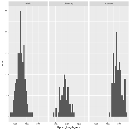That looks reasonable.

And the residuals?

R

aov(flipper_length_mm ~ species, data = penguins)$residuals %>% 
  hist(.)

That looks fine - if we want a more specific test, those exists, but will not be covered here.

Homoskedacity

A weird name, it simply means that the variance in the different groups are more or less the same. We can calculate the variance and compare:

R

penguins %>% 
  group_by(species) %>% 
  summarise(variance = var(flipper_length_mm, na.rm = TRUE))

OUTPUT

# A tibble: 3 × 2
  species   variance
  <fct>        <dbl>
1 Adelie        42.8
2 Chinstrap     50.9
3 Gentoo        42.1

Are the variances too different? As a rule of thumb, we have a problem if the largest variance is more than 4-5 times larger than the smallest variance. This is OK for this example.

If there is too large difference in the size of the three groups, smaller differences in variance can be problematic.

More specific methods exist.

There are probably more than than three tests for homoskedacity, here are three:

Fligner-Killeen test:

R

fligner.test(flipper_length_mm ~ species, data = penguins)

OUTPUT


	Fligner-Killeen test of homogeneity of variances

data:  flipper_length_mm by species
Fligner-Killeen:med chi-squared = 0.69172, df = 2, p-value = 0.7076

Bartlett’s test:

R

bartlett.test(flipper_length_mm ~ species, data = penguins)

OUTPUT


	Bartlett test of homogeneity of variances

data:  flipper_length_mm by species
Bartlett's K-squared = 0.91722, df = 2, p-value = 0.6322

Levene test:

R

library(car)

OUTPUT

Loading required package: carData

OUTPUT


Attaching package: 'car'

OUTPUT

The following object is masked from 'package:dplyr':

    recode

OUTPUT

The following object is masked from 'package:purrr':

    some

R

leveneTest(flipper_length_mm ~ species, data = penguins)

OUTPUT

Levene's Test for Homogeneity of Variance (center = median)
       Df F value Pr(>F)
group   2  0.3306 0.7188
      339

For all three tests - if the p-value is >0.05, there is a significant difference in the variance - and we are not allowed to use the ANOVA-method. In this case we are on the safe side.

But where is the difference?

Yes, there is a difference between the average flipper length of the three species. But that might arise from one of the species having extremely long flippers, and there not being much difference between the two other species.

So we do a posthoc analysis to confirm where the differences are.

The most common is the tukeyHSD test, HSD standing for “Honest Significant Differences”. We do that by saving the result of our ANOVa-analysis and run the TukeyHSD() function on the result:

R

aov_model <- aov(flipper_length_mm ~ species, data = penguins)

TukeyHSD(aov_model)

OUTPUT

  Tukey multiple comparisons of means
    95% family-wise confidence level

Fit: aov(formula = flipper_length_mm ~ species, data = penguins)

$species
                      diff       lwr       upr p adj
Chinstrap-Adelie  5.869887  3.586583  8.153191     0
Gentoo-Adelie    27.233349 25.334376 29.132323     0
Gentoo-Chinstrap 21.363462 19.000841 23.726084     0

We get the estimate of the pair-wise differences and lower and upper 95% confidence intervals for those differences.

Try it on your own

The iris dataset, build into R, contains measurements of three different species of the iris-family of flowers.

Is there a significant difference between the Sepal.Width of the three species?

Show me the solution

R

aov(Sepal.Width ~Species, data = iris) %>% 
  summary()

OUTPUT

             Df Sum Sq Mean Sq F value Pr(>F)
Species       2  11.35   5.672   49.16 <2e-16 ***
Residuals   147  16.96   0.115
---
Signif. codes:  0 '***' 0.001 '**' 0.01 '*' 0.05 '.' 0.1 ' ' 1

Try it on your own (continued)

The result only reveal that there is a difference. Or rather that we can reject the hypothesis that there is no difference.

Which species differ?

Show me the solution

R

aov(Sepal.Width ~Species, data = iris) %>% 
  TukeyHSD()

OUTPUT

  Tukey multiple comparisons of means
    95% family-wise confidence level

Fit: aov(formula = Sepal.Width ~ Species, data = iris)

$Species
                       diff         lwr        upr     p adj
versicolor-setosa    -0.658 -0.81885528 -0.4971447 0.0000000
virginica-setosa     -0.454 -0.61485528 -0.2931447 0.0000000
virginica-versicolor  0.204  0.04314472  0.3648553 0.0087802

Key Points

Use .md files for episodes when you want static content