Statistical tests
Last updated on 2026-06-15 | Edit this page
Overview
Questions
- How do I run X statistical test?
Objectives
- Provide a description on how to run common statistical tests
A collection of statistical tests
For all tests, the approach is:
- Formulate hypotheses
- Calculate test statistic
- Determine p-value
- Make decision
The cutoff chosen for all tests is a p-value of 0.05 unless otherwise indicated.
If a specific test is prefaced with “EJ KORREKTURLÆST” the text, examples etc have not been checked.
One sample tests
Or, more complete - one-sample chi-square goodnes-of-fit test.
- Used for: Testing whether observed categorical frequencies differ from expected frequencies under a specified distribution.
- Real-world example: Mars Inc. claims a specific distribution of colours in their M&M bags. Do the observed proportions in a given bag match their claim?
Assumptions
- Observations are independent.
- Categories are mutually exclusive and collectively exhaustive.
- Expected count in each category is at least 5 (for the chi-square approximation to be valid). The observed counts can be smaller, it is the expected counts that are important.
Strengths
- Simple to compute and interpret.
- Does not require the data to be normally distributed.
- Applicable to any number of categories.
Weaknesses
- Sensitive to small expected counts.
- Does not indicate which categories contribute most to the discrepancy without further investigation.
- Requires independence; cannot be used for paired or repeated measures.
Example
-
Null hypothesis (H₀): The proportions of M&M
colours equal the manufacturer’s claimed distribution.
- Alternative hypothesis (H₁): The proportion of at least one colour differs from the claimed distribution.
R
# Observed counts of M&M colors:
observed <- c(red = 20, blue = 25, green = 15, brown = 18, orange = 12, yellow = 10)

# Manufacturer's claimed proportions.
p_expected <- c(red = 0.12, blue = 0.24, green = 0.16, brown = 0.14, orange = 0.20, yellow = 0.14)

# Perform one-sample chi-square goodness-of-fit test:
test_result <- chisq.test(x = observed, p = p_expected)

# Display results:
test_result
OUTPUT
	Chi-squared test for given probabilities

data:  observed
X-squared = 10.923, df = 5, p-value = 0.05292Interpretation: The test yields χ² = 10.9 with a p-value = 0.05292. We fail to reject the null hypothesis, and there is no evidence to conclude a difference from the claimed distribution.
Note that in this example, the number of observations sums to 100.
chisq.test() normalises the expected values, so we do not
have to match the numbers.
-
Used for: Testing whether the mean of a single
sample differs from a known population mean when the population standard
deviation is known.
- Real-world example: Checking if the average diameter of manufactured ball bearings equals the specified 5.00 cm when σ is known. It can differ in three ways. It can differ from the specification. That is a Two-sided test. It can be smaller, that is a (left side) One-sided test. And it can be larger, that is a (right side) One-sided test.
Assumptions
- Sample is a simple random sample from the population.
- Observations are independent.
- Population standard deviation (σ) is known.
- The sampling distribution of the mean is approximately normal (either the population is normal or n is large, e.g. ≥ 30).
Strengths
- More powerful than the t-test when σ is truly known.
- Simple calculation and interpretation.
Weaknesses
- The true population σ is only very rarely known in practice.
- Sensitive to departures from normality for small samples.
- Misspecification of σ leads to incorrect inferences.
Example
Two-sided:
-
Null hypothesis (H₀): The true mean diameter μ =
5.00 cm.
- Alternative hypothesis (H₁): μ ≠ 5.00 cm.
One-sided, left:
-
Null hypothesis (H₀): The true mean diameter μ =
5.00 cm.
- Alternative hypothesis (H₁): μ < 5.00 cm.
One-sided, right:
-
Null hypothesis (H₀): The true mean diameter μ =
5.00 cm.
- Alternative hypothesis (H₁): μ > 5.00 cm.
R
# Sample of diameters (cm) for 25 ball bearings:
diameters <- c(5.03, 4.97, 5.01, 5.05, 4.99, 5.02, 5.00, 5.04, 4.96, 5.00,
               5.01, 4.98, 5.02, 5.03, 4.94, 5.00, 5.02, 4.99, 5.01, 5.03,
               4.98, 5.00, 5.04, 4.97, 5.02)

# Known population standard deviation:
sigma <- 0.05

# Hypothesized mean:
mu0 <- 5.00

# Compute test statistic:
n <- length(diameters)
xbar <- mean(diameters)
z_stat <- (xbar - mu0) / (sigma / sqrt(n))

# Two-sided p-value:
two_sided_p_value <- 2 * (1 - pnorm(abs(z_stat)))

# Larger p-value
p_value_larger_mu <- 1- pnorm(z_stat)

# Smaller p-value
p_value_smaller_mu <- pnorm(z_stat)

# Output results:
z_stat; two_sided_p_value; p_value_larger_mu; p_value_smaller_mu
OUTPUT
[1] 0.44OUTPUT
[1] 0.6599371OUTPUT
[1] 0.3299686OUTPUT
[1] 0.6700314Interpretation:
The sample mean is 5.004 cm. The z-statistic is 0.44 with a two-sided p-value of 0.66. We fail to reject the null hypothesis. Thus, there is no evidence to conclude a difference from the specified diameter of 5.00 cm.
We can similarly reject the hypothesis that the average diameter is larger (p = 0.3299686) or that it is smaller (p = 0.6700314)
EJ KORREKTURLÆST!
Her kan vi nok med fordel bruge samme eksempel som i z-testen.
-
Used for: Testing whether the mean of a single
sample differs from a known or hypothesized population mean when the
population standard deviation is unknown.
- Real-world example: Determining if the average exam score of a class differs from the passing threshold of 70%.
Assumptions:
- Sample is a simple random sample from the population.
- Observations are independent.
- The data are approximately normally distributed (especially important for small samples; n ≥ 30 reduces sensitivity).
Strengths: * Does not require knowing the population
standard deviation.
* Robust to mild departures from normality for moderate-to-large sample
sizes.
* Widely applicable and easily implemented.
Weaknesses * Sensitive to outliers in small
samples.
* Performance degrades if normality assumption is seriously violated and
n is small.
* Degrees of freedom reduce power relative to z-test.
Example
-
Null hypothesis (H₀): The true mean exam score μ =
70.
- Alternative hypothesis (H₁): μ ≠ 70.
R
# Sample of exam scores for 20 students:
scores <- c(68, 74, 71, 69, 73, 65, 77, 72, 70, 66,
            75, 68, 71, 69, 74, 67, 72, 70, 73, 68)

# Hypothesized mean:
mu0 <- 70

# Perform one-sample t-test:
test_result <- t.test(x = scores, mu = mu0)

# Display results:
test_result
OUTPUT
	One Sample t-test

data:  scores
t = 0.84675, df = 19, p-value = 0.4077
alternative hypothesis: true mean is not equal to 70
95 percent confidence interval:
 69.1169 72.0831
sample estimates:
mean of x
     70.6
Interpretation:
The sample mean is 70.6. The t-statistic is 0.85 with 19 degrees of freedom and a two-sided p-value of 0.408. We fail to reject the null hypothesis. Thus, there is no evidence to conclude the average score differs from the passing threshold of 70.
EJ KORREKTURLÆST!
-
Used for Testing whether the observed count of
events in a fixed period differs from a hypothesized Poisson rate.
- Real-world example: Checking if the number of customer arrivals per hour at a call center matches the expected rate of 30 calls/hour.
Assumptions * Events occur independently.
* The rate of occurrence (λ) is constant over the observation
period.
* The count of events in non-overlapping intervals is independent.
Strengths * Exact test based on the Poisson
distribution (no large-sample approximation needed).
* Valid for small counts and rare events.
* Simple to implement in R via poisson.test().
Weaknesses * Sensitive to violations of the Poisson
assumptions (e.g., overdispersion or time-varying rate).
* Only assesses the overall rate, not the dispersion or clustering of
events.
* Cannot handle covariates or more complex rate structures.
Example
-
Null hypothesis (H₀): The event rate λ = 30
calls/hour.
- Alternative hypothesis (H₁): λ ≠ 30 calls/hour.
R
# Observed number of calls in one hour:
observed_calls <- 36

# Hypothesized rate (calls per hour):
lambda0 <- 30

# Perform one-sample Poisson test (two-sided):
test_result <- poisson.test(x = observed_calls, T = 1, r = lambda0, alternative = "two.sided")

# Display results:
test_result
OUTPUT
	Exact Poisson test

data:  observed_calls time base: 1
number of events = 36, time base = 1, p-value = 0.272
alternative hypothesis: true event rate is not equal to 30
95 percent confidence interval:
 25.21396 49.83917
sample estimates:
event rate
        36
Interpretation:
The test reports an observed count of 36 calls versus an expected 30 calls, yielding a p-value of 0.272. We fail to reject the null hypothesis. Thus, there is no evidence to conclude the call rate differs from 30 calls/hour.
EJ KORREKTURLÆST. DEN HAR VI NOGET UNDERVISNINGSMATERIALE OM I “ER DET NORMALT?”
-
Used for Testing whether a sample comes from a
normally distributed population.
- Real-world example: Checking if the distribution of daily blood glucose measurements in a patient cohort is approximately normal.
Assumptions * Observations are independent.
* Data are continuous.
* No extreme ties or many identical values.
Strengths * Good power for detecting departures from
normality in small to moderate samples (n ≤ 50).
* Widely implemented and easy to run in R.
* Provides both a test statistic (W) and p-value.
Weaknesses * Very sensitive to even slight
deviations from normality in large samples (n > 2000).
* Does not indicate the nature of the departure (e.g., skewness
vs. kurtosis).
* Ties or repeated values can invalidate the test.
Example
-
Null hypothesis (H₀): The sample is drawn from a
normal distribution.
- Alternative hypothesis (H₁): The sample is not drawn from a normal distribution.
R
# Simulate a sample of 30 observations from a normal distribution:
set.seed(123)
sample_data <- rnorm(30, mean = 100, sd = 15)

# Perform Shapiro–Wilk test:
sw_result <- shapiro.test(sample_data)

# Display results:
sw_result
OUTPUT
	Shapiro-Wilk normality test

data:  sample_data
W = 0.97894, p-value = 0.7966
Interpretation:
The Shapiro–Wilk statistic W = 0.979 with p-value = 0.797. We fail to reject the null hypothesis. Thus, there is no evidence to conclude a departure from normality.
EJ KORREKTURLÆST. DENNE HAR VI OGSÅ UNDERVISNINGSMATERIALE OM I “ER DET NORMALT”
-
Used for Testing whether a sample comes from a
specified continuous distribution.
- Real-world example: Checking if patient systolic blood pressures follow a normal distribution with mean 120 mmHg and SD 15 mmHg.
Assumptions * Observations are independent.
* Data are continuous (no ties).
* The null distribution is fully specified (parameters known, not
estimated from the data).
Strengths * Nonparametric: makes no assumption about
distribution shape beyond continuity.
* Sensitive to any kind of departure (location, scale, shape).
* Exact distribution of the test statistic under H₀.
Weaknesses * Requires that distribution parameters
(e.g., mean, SD) are known a priori; if estimated from data, p-values
are invalid.
* Less powerful than parametric tests when the parametric form is
correct.
* Sensitive to ties and discrete data.
Example
-
Null hypothesis (H₀): The blood pressure values
follow a Normal(μ = 120, σ = 15) distribution.
- Alternative hypothesis (H₁): The blood pressure values do not follow Normal(120, 15).
R
set.seed(2025)
# Simulate systolic blood pressure for 40 patients:
sample_bp <- rnorm(40, mean = 120, sd = 15)

# Perform one-sample Kolmogorov–Smirnov test against N(120,15):
ks_result <- ks.test(sample_bp, "pnorm", mean = 120, sd = 15)

# Show results:
ks_result
OUTPUT
	Exact one-sample Kolmogorov-Smirnov test

data:  sample_bp
D = 0.11189, p-value = 0.6573
alternative hypothesis: two-sided
Interpretation:
The KS statistic D = 0.112 with p-value = 0.657. We fail to reject the null hypothesis. Thus, there is no evidence to conclude deviation from Normal(120,15).
EJ KORREKTURLÆST
-
Used for Testing whether observed categorical
frequencies differ from expected categorical proportions.
- Real-world example: Comparing the distribution of blood types in a sample of donors to known population proportions.
Assumptions * Observations are independent.
* Categories are mutually exclusive and exhaustive.
* Expected count in each category is at least 5 for the chi-square
approximation to hold.
Strengths * Simple to compute and interpret.
* Nonparametric: no requirement of normality.
* Flexible for any number of categories.
Weaknesses * Sensitive to small expected counts
(invalidates approximation).
* Doesn’t identify which categories drive the discrepancy without
further post-hoc tests.
* Requires independence—unsuitable for paired or repeated measures.
Example
-
Null hypothesis (H₀): The sample blood type
proportions equal the known population proportions (A=0.42, B=0.10,
AB=0.04, O=0.44).
- Alternative hypothesis (H₁): At least one blood type proportion differs from its known value.
R
# Observed counts of blood types in 200 donors:
observed <- c(A = 85, B = 18, AB = 6, O = 91)

# Known population proportions:
p_expected <- c(A = 0.42, B = 0.10, AB = 0.04, O = 0.44)

# Perform chi-square goodness-of-fit test:
test_result <- chisq.test(x = observed, p = p_expected)

# Display results:
test_result
OUTPUT
	Chi-squared test for given probabilities

data:  observed
X-squared = 0.81418, df = 3, p-value = 0.8461
Interpretation:
The test yields χ² = 0.81 with p-value = 0.846. We fail to reject the null hypothesis. Thus, there is no evidence to conclude the sample proportions differ from the population.
To-prøve-tests og parrede tests
EJ KORREKTURLÆST
We use this when we want to determine if two independent samples originate from populations with the same variance.
-
Used for Testing whether two independent samples
have equal variances.
- Real-world example: Comparing the variability in systolic blood pressure measurements between two clinics.
Assumptions * Both samples consist of independent
observations.
* Each sample is drawn from a normally distributed population.
* Samples are independent of one another.
Strengths * Simple calculation and
interpretation.
* Directly targets variance equality, a key assumption in many
downstream tests (e.g., t-test).
* Exact inference under normality.
Weaknesses * Highly sensitive to departures from
normality.
* Only compares variance—doesn’t assess other distributional
differences.
* Not robust to outliers.
Example
-
Null hypothesis (H₀): σ₁² = σ₂² (the two population
variances are equal).
- Alternative hypothesis (H₁): σ₁² ≠ σ₂² (the variances differ).
R
# Simulate systolic BP (mmHg) from two clinics:
set.seed(2025)
clinicA <- rnorm(30, mean = 120, sd = 8)
clinicB <- rnorm(25, mean = 118, sd = 12)

# Perform two-sample F-test for variances:
f_result <- var.test(clinicA, clinicB, alternative = "two.sided")

# Display results:
f_result
OUTPUT
	F test to compare two variances

data:  clinicA and clinicB
F = 0.41748, num df = 29, denom df = 24, p-value = 0.02606
alternative hypothesis: true ratio of variances is not equal to 1
95 percent confidence interval:
 0.1882726 0.8992623
sample estimates:
ratio of variances
         0.4174837
Interpretation
The F statistic is 0.417 with numerator df = 29 and denominator df = 24, and p-value = 0.0261. We
reject the null hypothesis. Thus, there is evidence that the variability in blood pressure differs between the two clinics.
EJ KORREKTURLÆST
-
Used for Testing whether the mean difference
between two related (paired) samples differs from zero.
- Real-world example: Comparing patients’ blood pressure before and after administering a new medication.
Assumptions * Paired observations are independent of
other pairs.
* Differences between pairs are approximately normally
distributed.
* The scale of measurement is continuous (interval or ratio).
Strengths * Controls for between‐subject variability
by using each subject as their own control.
* More powerful than unpaired tests when pairs are truly
dependent.
* Easy to implement and interpret.
Weaknesses * Sensitive to outliers in the difference
scores.
* Requires that differences be approximately normal, especially for
small samples.
* Not appropriate if pairing is not justified or if missing data break
pairs.
Example
-
Null hypothesis (H₀): The mean difference Δ = 0 (no
change in blood pressure).
- Alternative hypothesis (H₁): Δ ≠ 0 (blood pressure changes after medication).
R
# Simulated systolic blood pressure (mmHg) for 15 patients before and after treatment:
before <- c(142, 138, 150, 145, 133, 140, 147, 139, 141, 136, 144, 137, 148, 142, 139)
after  <- c(135, 132, 144, 138, 128, 135, 142, 133, 136, 130, 139, 132, 143, 137, 133)

# Perform paired t-test:
test_result <- t.test(before, after, paired = TRUE)

# Display results:
test_result
OUTPUT
	Paired t-test

data:  before and after
t = 29.437, df = 14, p-value = 5.418e-14
alternative hypothesis: true mean difference is not equal to 0
95 percent confidence interval:
 5.19198 6.00802
sample estimates:
mean difference
            5.6
Interpretation:
The mean difference (before – after) is 5.6 mmHg. The t‐statistic is
29.44 with 14 degrees of freedom and a two‐sided p‐value
ofr signif(test_result$p.value, 3). We reject the null
hypothesis. Thus, there is evidence that the medication significantly
changed blood pressure.
EJ KORREKTURLÆST
- Used for Testing whether the means of two independent samples differ, assuming equal variances.
- Real-world example: Comparing average systolic blood pressure between male and female patients when variability is similar.
Assumptions * Observations in each group are
independent.
* Both populations are normally distributed (especially important for
small samples).
* The two populations have equal variances (homoscedasticity).
Strengths * More powerful than Welch’s t-test when
variances truly are equal.
* Simple computation and interpretation via pooled variance.
* Widely implemented and familiar to practitioners.
Weaknesses * Sensitive to violations of normality in
small samples.
* Incorrect if variances differ substantially—can inflate Type I
error.
* Assumes homogeneity of variance, which may not hold in practice.
Example
-
Null hypothesis (H₀): μ₁ = μ₂ (the two population
means are equal).
- Alternative hypothesis (H₁): μ₁ ≠ μ₂ (the means differ).
R
set.seed(2025)
# Simulate systolic BP (mmHg):
groupA <- rnorm(25, mean = 122, sd = 10)  # e.g., males
groupB <- rnorm(25, mean = 118, sd = 10)  # e.g., females

# Perform two-sample t-test with equal variances:
test_result <- t.test(groupA, groupB, var.equal = TRUE)

# Display results:
test_result
OUTPUT
	Two Sample t-test

data:  groupA and groupB
t = 2.6245, df = 48, p-value = 0.0116
alternative hypothesis: true difference in means is not equal to 0
95 percent confidence interval:
  1.733091 13.086377
sample estimates:
mean of x mean of y
 125.2119  117.8021
Interpretation:
The pooled estimate of the difference in means is 7.41 mmHg. The t-statistic is 2.62 with df = 48 and p-value = 0.0116. We reject the null hypothesis. Thus, there is evidence that the average systolic blood pressure differs between the two groups.
EJ KORREKTURLÆST
Used for Testing whether the means of two
independent samples differ when variances are unequal.
* Real-world example: Comparing average recovery times
for two different therapies when one therapy shows more variable
outcomes.
Assumptions * Observations in each group are
independent.
* Each population is approximately normally distributed (especially
important for small samples).
* Does not assume equal variances across groups.
Strengths * Controls Type I error when variances
differ.
* More reliable than the pooled‐variance t‐test under
heteroskedasticity.
* Simple to implement via t.test(..., var.equal = FALSE) in
R.
Weaknesses * Slight loss of power compared to
equal-variance t‐test when variances truly are equal.
* Sensitive to departures from normality in small samples.
* Degrees of freedom are approximated (Welch–Satterthwaite), which can
reduce interpretability.
Example
-
Null hypothesis (H₀): μ₁ = μ₂ (the two population
means are equal).
- Alternative hypothesis (H₁): μ₁ ≠ μ₂ (the means differ).
R
set.seed(2025)
# Simulate recovery times (days) for two therapies:
therapyA <- rnorm(20, mean = 10, sd = 2)   # Therapy A
therapyB <- rnorm(25, mean = 12, sd = 4)   # Therapy B (more variable)

# Perform two-sample t-test with unequal variances:
test_result <- t.test(therapyA, therapyB, var.equal = FALSE)

# Display results:
test_result
OUTPUT
	Welch Two Sample t-test

data:  therapyA and therapyB
t = -1.7792, df = 32.794, p-value = 0.08449
alternative hypothesis: true difference in means is not equal to 0
95 percent confidence interval:
 -3.8148079  0.2558875
sample estimates:
mean of x mean of y
 10.41320  12.19266
Interpretation:
The estimated difference in means is -1.78 days. The Welch
t‐statistic isr round(test_result$statistic, 2) with df ≈
32.8 and two‐sided p‐value
=r signif(test_result$p.value, 3). We fail to reject the
null hypothesis. Thus, there is no evidence of a difference in average
recovery times..
EJ KORREKTURLÆST
-
Used for Comparing the central tendencies of two
independent samples when the data are ordinal or not normally
distributed.
- Real-world example: Testing whether pain scores (0–10) differ between patients receiving Drug A versus Drug B when scores are skewed.
Assumptions * Observations are independent both
within and between groups.
* The response variable is at least ordinal.
* The two distributions have the same shape (so that differences reflect
location shifts).
Strengths * Nonparametric: does not require
normality or equal variances.
* Robust to outliers and skewed data.
* Simple rank-based calculation.
Weaknesses * Less powerful than t-test when data are
truly normal.
* If distributions differ in shape as well as location, interpretation
becomes ambiguous.
* Only tests for location shift, not differences in dispersion.
Example
-
Null hypothesis (H₀): The distributions of pain
scores are identical for Drug A and Drug B.
- Alternative hypothesis (H₁): The distributions differ in location (median pain differs between drugs).
R
# Simulate pain scores (0–10) for two independent groups:
set.seed(2025)
drugA <- c(2,3,4,5,4,3,2,6,5,4,  # skewed lower
           3,4,5,4,3,2,3,4,5,3)
drugB <- c(4,5,6,7,6,5,7,8,6,7,  # skewed higher
           6,7,5,6,7,6,8,7,6,7)

# Perform Mann–Whitney U test (Wilcoxon rank-sum):
mw_result <- wilcox.test(drugA, drugB, alternative = "two.sided", exact = FALSE)

# Display results:
mw_result
OUTPUT
	Wilcoxon rank sum test with continuity correction

data:  drugA and drugB
W = 20.5, p-value = 9.123e-07
alternative hypothesis: true location shift is not equal to 0
Interpretation:
The Wilcoxon rank-sum statistic W = 20.5 with p-value = 9.12^{-7}. We reject the null hypothesis. Thus, there is evidence that median pain scores differ between Drug A and Drug B.
EJ KORREKTURLÆST
-
Used for Testing whether the median difference
between paired observations is zero.
- Real-world example: Comparing patients’ pain scores before and after a new analgesic treatment when differences may not be normally distributed.
Assumptions * Observations are paired and the pairs
are independent.
* Differences are at least ordinal and symmetrically distributed around
the median.
* No large number of exact zero differences (ties).
Strengths * Nonparametric: does not require
normality of differences.
* Controls for within‐subject variability by using paired design.
* Robust to outliers in the paired differences.
Weaknesses * Less powerful than the paired t-test
when differences are truly normal.
* Requires symmetry of the distribution of differences.
* Cannot easily handle many tied differences.
Example
-
Null hypothesis (H₀): The median difference in pain
score (before – after) = 0 (no change).
- Alternative hypothesis (H₁): The median difference ≠ 0 (pain changes after treatment).
R
# Simulated pain scores (0–10) for 12 patients:
before <- c(6, 7, 5, 8, 6, 7, 9, 5, 6, 8, 7, 6)
after  <- c(4, 6, 5, 7, 5, 6, 8, 4, 5, 7, 6, 5)

# Perform Wilcoxon signed-rank test:
wsr_result <- wilcox.test(before, after, paired = TRUE,
                          alternative = "two.sided", exact = FALSE)

# Display results:
wsr_result
OUTPUT
	Wilcoxon signed rank test with continuity correction

data:  before and after
V = 66, p-value = 0.001586
alternative hypothesis: true location shift is not equal to 0
Interpretation:
The Wilcoxon signed‐rank test statistic V =66 with p-value
=r signif(wsr_result$p.value, 3). We reject the null
hypothesis. Thus, there is evidence that median pain scores change after
treatment..
EJ KORREKTURLÆST
-
Used for Testing whether two independent samples
come from the same continuous distribution.
- Real-world example: Comparing the distribution of recovery times for patients receiving Drug A versus Drug B.
Assumptions * Observations in each sample are
independent.
* Data are continuous with no ties.
* The two samples are drawn from fully specified continuous
distributions (no parameters estimated from the same data).
Strengths * Nonparametric: makes no assumption about
the shape of the distribution.
* Sensitive to differences in location, scale, or overall shape.
* Exact distribution under the null when samples are not too large.
Weaknesses * Less powerful than parametric
alternatives if the true form is known (e.g., t-test for normal
data).
* Invalid p-values if there are ties or discrete data.
* Does not indicate how distributions differ—only that they do.
Example
-
Null hypothesis (H₀): The two samples come from the
same distribution.
- Alternative hypothesis (H₁): The two samples come from different distributions.
R
# Simulate recovery times (days) for two therapies:
set.seed(2025)
therapyA <- rnorm(30, mean = 10, sd = 2)   # Therapy A
therapyB <- rnorm(30, mean = 12, sd = 3)   # Therapy B

# Perform two-sample Kolmogorov–Smirnov test:
ks_result <- ks.test(therapyA, therapyB, alternative = "two.sided", exact = FALSE)

# Display results:
ks_result
OUTPUT
	Asymptotic two-sample Kolmogorov-Smirnov test

data:  therapyA and therapyB
D = 0.43333, p-value = 0.007153
alternative hypothesis: two-sided
Interpretation:
The KS statistic D = 0.433 with p-value = 0.00715. We reject the null hypothesis. Thus, there is evidence that the distribution of recovery times differs between therapies.
EJ KORREKTURLÆST
-
Used for Testing whether multiple groups have equal
variances.
- Real-world example: Checking if the variability in patient blood pressure differs between three different clinics.
Assumptions
- Observations are independent.
- The underlying distributions within each group are approximately symmetric (Levene’s test is robust to non-normality but assumes no extreme skew).
Strengths * More robust to departures from normality
than Bartlett’s test.
* Applicable to two or more groups.
* Simple to implement and interpret.
Weaknesses * Less powerful than tests that assume
normality when data truly are normal.
* Can be sensitive to extreme outliers despite its robustness.
* Does not indicate which groups differ in variance without follow-up
comparisons.
Example
-
Null hypothesis (H₀): All groups have equal
variances (σ₁² = σ₂² = … = σₖ²).
- Alternative hypothesis (H₁): At least one group’s variance differs.
R
# Simulate data for three groups (n = 10 each):
set.seed(123)
group   <- factor(rep(c("ClinicA", "ClinicB", "ClinicC"), each = 10))
scores  <- c(rnorm(10, mean = 120, sd = 5),
             rnorm(10, mean = 120, sd = 8),
             rnorm(10, mean = 120, sd = 5))
df      <- data.frame(group, scores)

# Perform Levene’s test for homogeneity of variances:
library(car)
OUTPUT
Loading required package: carDataR
levene_result <- leveneTest(scores ~ group, data = df)

# Show results:
levene_result
OUTPUT
Levene's Test for Homogeneity of Variance (center = median)
      Df F value Pr(>F)
group  2   0.872 0.4296
      27
Interpretation:
Levene’s test yields an F-statistic of 0.87 with a p-value of 0.43. We fail to reject the null hypothesis. This means there is no evidence of differing variances across clinics.
EJ KORREKTURLÆST
-
Used for Testing whether multiple groups have equal
variances under the assumption of normality.
- Real-world example: Checking if the variability in laboratory test results differs across three different laboratories.
Assumptions * Observations within each group are
independent.
* Each group is drawn from a normally distributed population.
* Groups are independent of one another.
Strengths * More powerful than Levene’s test when
normality holds.
* Directly targets equality of variances under the normal model.
* Simple to compute in R via bartlett.test().
Weaknesses * Highly sensitive to departures from
normality—small deviations can inflate Type I error.
* Does not indicate which groups differ without further pairwise
testing.
* Not robust to outliers.
Example
-
Null hypothesis (H₀): All group variances are equal
(σ₁² = σ₂² = σ₃²).
- Alternative hypothesis (H₁): At least one group variance differs.
R
# Simulate data for three laboratories (n = 12 each):
set.seed(456)
lab      <- factor(rep(c("LabA", "LabB", "LabC"), each = 12))
values   <- c(rnorm(12, mean = 100, sd = 5),
              rnorm(12, mean = 100, sd = 8),
              rnorm(12, mean = 100, sd = 5))
df       <- data.frame(lab, values)

# Perform Bartlett’s test for homogeneity of variances:
bartlett_result <- bartlett.test(values ~ lab, data = df)

# Display results:
bartlett_result
OUTPUT
	Bartlett test of homogeneity of variances

data:  values by lab
Bartlett's K-squared = 10.387, df = 2, p-value = 0.005552
Interpretation:
Bartlett’s K-squared = 10.39 with df = 2 and p-value = 0.00555. We reject the null hypothesis. Thus, there is evidence that at least one laboratory’s variance differs from the others.
Variansanalyse (ANOVA/ANCOVA)
EJ KORREKTURLÆST
SAMMENHOLD MED undervisningsudgaven
-
Used for Testing whether the means of three or more
independent groups differ.
- Real-world example: Comparing average test scores among students taught by three different teaching methods.
Assumptions * Observations are independent.
* Each group’s residuals are approximately normally distributed.
* Homogeneity of variances across groups.
Strengths * Controls Type I error rate when
comparing multiple groups.
* Simple to compute and interpret via F-statistic.
* Foundation for many extensions (e.g., factorial ANOVA, mixed
models).
Weaknesses * Sensitive to heterogeneity of
variances, especially with unequal group sizes.
* Only tells you that at least one mean differs—does not indicate which
groups differ without post-hoc tests.
* Assumes normality; moderately robust for large samples, but small
samples can be problematic.
Example
-
Null hypothesis (H₀): μ₁ = μ₂ = μ₃ (all three group
means are equal).
- Alternative hypothesis (H₁): At least one group mean differs.
R
# Simulate exam scores for three teaching methods (n = 20 each):
set.seed(2025)
method <- factor(rep(c("Lecture", "Online", "Hybrid"), each = 20))
scores <- c(rnorm(20, mean = 75, sd = 8),
            rnorm(20, mean = 80, sd = 8),
            rnorm(20, mean = 78, sd = 8))
df     <- data.frame(method, scores)

# Fit one-way ANOVA:
anova_fit <- aov(scores ~ method, data = df)

# Summarize ANOVA table:
anova_summary <- summary(anova_fit)
anova_summary
OUTPUT
            Df Sum Sq Mean Sq F value Pr(>F)
method       2    146   72.79   1.184  0.314
Residuals   57   3505   61.48
Interpretation:
The ANOVA yields F = 1.18 with df₁
=r anova_summary[[1]]["method","Df"] and df₂
=r anova_summary[[1]]["Residuals","Df"], and p-value =
0.314. We fail to reject the null hypothesis. Thus, there is no evidence
of a difference in mean scores among methods.
EJ KORREKTURLÆST
-
Used for Comparing group means on a continuous
outcome while adjusting for one continuous covariate.
- Real-world example: Evaluating whether three different teaching methods lead to different final exam scores after accounting for students’ prior GPA.
Assumptions * Observations are independent.
* The relationship between the covariate and the outcome is linear and
the same across groups (homogeneity of regression slopes).
* Residuals are normally distributed with equal variances across
groups.
* Covariate is measured without error and is independent of group
assignment.
Strengths * Removes variability due to the
covariate, increasing power to detect group differences.
* Controls for confounding by the covariate.
* Simple extension of one-way ANOVA with interpretation familiar to
ANOVA users.
Weaknesses * Sensitive to violation of homogeneity
of regression slopes.
* Mis‐specification of the covariate‐outcome relationship biases
results.
* Requires accurate measurement of the covariate.
* Does not accommodate multiple covariates without extension to
factorial ANCOVA or regression.
Example
-
Null hypothesis (H₀): After adjusting for prior
GPA, the mean final exam scores are equal across the three teaching
methods (μ_Lecture = μ_Online = μ_Hybrid).
- Alternative hypothesis (H₁): At least one adjusted group mean differs.
R
set.seed(2025)
n <- 20
method <- factor(rep(c("Lecture","Online","Hybrid"), each = n))
prior_gpa <- rnorm(3*n, mean = 3.0, sd = 0.3)

# Simulate final exam scores with a covariate effect:
# true intercepts 75, 78, 80; slope = 5 points per GPA unit; noise sd = 5
final_score <- 75 +
               ifelse(method=="Online", 3, 0) +
               ifelse(method=="Hybrid", 5, 0) +
               5 * prior_gpa +
               rnorm(3*n, sd = 5)

df <- data.frame(method, prior_gpa, final_score)

# Fit one-way ANCOVA:
ancova_fit <- aov(final_score ~ prior_gpa + method, data = df)
ancova_summary <- summary(ancova_fit)
ancova_summary
OUTPUT
            Df Sum Sq Mean Sq F value  Pr(>F)
prior_gpa    1  166.5   166.5   5.967 0.01775 *
method       2  296.8   148.4   5.320 0.00767 **
Residuals   56 1562.4    27.9
---
Signif. codes:  0 '***' 0.001 '**' 0.01 '*' 0.05 '.' 0.1 ' ' 1
Interpretation:
After adjusting for prior GPA, the effect of teaching method yields F
= 5.32 (df₁ =r ancova_summary[[1]]["method","Df"], df₂
=r ancova_summary[[1]]["Residuals","Df"]) with p
=r signif(ancova_summary[[1]]["method","Pr(>F)"], 3). We
reject the null hypothesis. Thus, there is evidence that, controlling
for prior GPA, at least one teaching method leads to a different average
final score..
EJ KORREKTURLÆST
-
Used for Testing whether the means of three or more
independent groups differ when variances are unequal.
- Real-world example: Comparing average systolic blood pressure across three clinics known to have different measurement variability.
Assumptions * Observations are independent.
* Each group’s residuals are approximately normally distributed.
* Does not assume equal variances across groups.
Strengths * Controls Type I error under
heteroskedasticity better than ordinary ANOVA.
* Simple to implement via
oneway.test(..., var.equal = FALSE).
* More powerful than nonparametric alternatives when normality
holds.
Weaknesses * Sensitive to departures from normality,
especially with small sample sizes.
* Does not provide post-hoc comparisons by default; requires additional
tests.
* Still assumes independence and approximate normality within each
group.
Example
-
Null hypothesis (H₀): All group means are equal (μ₁
= μ₂ = μ₃).
- Alternative hypothesis (H₁): At least one group mean differs.
R
set.seed(2025)
# Simulate systolic BP (mmHg) for three clinics with unequal variances:
clinic   <- factor(rep(c("A","B","C"), times = c(15, 20, 12)))
bp_values <- c(
  rnorm(15, mean = 120, sd = 5),
  rnorm(20, mean = 125, sd = 10),
  rnorm(12, mean = 118, sd = 7)
)
df <- data.frame(clinic, bp_values)

# Perform Welch’s one-way ANOVA:
welch_result <- oneway.test(bp_values ~ clinic, data = df, var.equal = FALSE)

# Display results:
welch_result
OUTPUT
	One-way analysis of means (not assuming equal variances)

data:  bp_values and clinic
F = 2.7802, num df = 2.000, denom df = 23.528, p-value = 0.08244
Interpretation:
The Welch statistic = 2.78 with df ≈ 2, 23.53, and p-value = 0.0824. We fail to reject the null hypothesis. Thus, there is no evidence of a difference in mean blood pressure among the clinics.
EJ KORREKTURLÆST
-
Used for Testing whether the means of three or more
related (within‐subject) conditions differ.
- Real-world example: Assessing whether students’ reaction times change across three levels of sleep deprivation (0 h, 12 h, 24 h) measured on the same individuals.
Assumptions * Observations (subjects) are
independent.
* The dependent variable is approximately normally distributed in each
condition.
* Sphericity: variances of the pairwise differences
between conditions are equal.
Strengths * Controls for between‐subject variability
by using each subject as their own control.
* More powerful than independent‐groups ANOVA when measures are
correlated.
* Can model complex within‐subject designs (e.g. time × treatment
interactions).
Weaknesses * Sensitive to violations of sphericity
(inflates Type I error).
* Missing data in any condition drops the entire subject (unless using
more advanced mixed‐model methods).
* Interpretation can be complex when there are many levels or
interactions.
Example
-
Null hypothesis (H₀): The mean reaction time is the
same across 0 h, 12 h, and 24 h sleep deprivation.
- Alternative hypothesis (H₁): At least one condition’s mean reaction time differs.
R
set.seed(2025)
n_subj <- 12
subject <- factor(rep(1:n_subj, each = 3))
condition <- factor(rep(c("0h","12h","24h"), times = n_subj))
# Simulate reaction times (ms):
rt <- c(rnorm(n_subj, mean = 300, sd = 20),
        rnorm(n_subj, mean = 320, sd = 20),
        rnorm(n_subj, mean = 340, sd = 20))
df <- data.frame(subject, condition, rt)

# Fit repeated-measures ANOVA:
rm_fit <- aov(rt ~ condition + Error(subject/condition), data = df)
rm_summary <- summary(rm_fit)

# Display results:
rm_summary
OUTPUT
Error: subject
          Df Sum Sq Mean Sq F value Pr(>F)
Residuals 11   9892   899.3

Error: subject:condition
          Df Sum Sq Mean Sq F value Pr(>F)
condition  2   1000     500   1.188  0.324
Residuals 22   9262     421
Interpretation:
The within‐subjects effect of sleep deprivation yields F = 1.19 with
df₁ = 2 and df₂ = r rm_summary[[2]][[1]]["Residuals","Df"],
p = 0.324. We fail to reject the null hypothesis. Thus, there is no
evidence that reaction times differ across sleep deprivation
conditions.
EJ KORREKTURLÆST
-
Used for Testing for differences on multiple
continuous dependent variables across one or more grouping factors
simultaneously.
- Real-world example: Evaluating whether three different diets lead to different patterns of weight loss and cholesterol reduction.
Assumptions * Multivariate normality of the
dependent variables within each group.
* Homogeneity of covariance matrices across groups.
* Observations are independent.
* Linear relationships among dependent variables.
Strengths * Controls family-wise Type I error by
testing all DVs together.
* Can detect patterns that univariate ANOVAs might miss.
* Provides multiple test statistics (Pillai, Wilks, Hotelling–Lawley,
Roy) for flexibility.
Weaknesses * Sensitive to violations of multivariate
normality and homogeneity of covariances.
* Requires larger sample sizes as the number of DVs increases.
* Interpretation can be complex; follow-up analyses often needed to
determine which DVs drive effects.
Example
-
Null hypothesis (H₀): The vector of means for
weight loss and cholesterol change is equal across the three diet
groups.
- Alternative hypothesis (H₁): At least one diet group differs on the combination of weight loss and cholesterol change.
R
set.seed(2025)
n_per_group <- 15
diet <- factor(rep(c("LowFat", "LowCarb", "Mediterranean"), each = n_per_group))

# Simulate outcomes:
weight_loss <- c(rnorm(n_per_group, mean = 5,  sd = 1.5),
                 rnorm(n_per_group, mean = 8,  sd = 1.5),
                 rnorm(n_per_group, mean = 7,  sd = 1.5))
cholesterol  <- c(rnorm(n_per_group, mean = 10, sd = 2),
                 rnorm(n_per_group, mean = 12, sd = 2),
                 rnorm(n_per_group, mean = 9,  sd = 2))

df <- data.frame(diet, weight_loss, cholesterol)

# Fit MANOVA:
manova_fit <- manova(cbind(weight_loss, cholesterol) ~ diet, data = df)

# Summarize using Pillai’s trace:
manova_summary <- summary(manova_fit, test = "Pillai")
manova_summary
OUTPUT
          Df  Pillai approx F num Df den Df    Pr(>F)
diet       2 0.58953   8.7773      4     84 5.708e-06 ***
Residuals 42
---
Signif. codes:  0 '***' 0.001 '**' 0.01 '*' 0.05 '.' 0.1 ' ' 1
Interpretation:
Pillai’s trace = 0.59, F = 8.78 with df = 42, and p-value = 5.71^{-6}. We reject the null hypothesis. This indicates that there is
a significant multivariate effect of diet on weight loss and cholesterol change.
Pillai?
Der er fire almindeligt brugte taststatistikker i MANOVA. Pillai, Wilks’ lambd, Hotelling-Lawleys trace og Roys largest root.
Pillai’s trace (også kaldet Pillai–Bartlett’s trace) er én af fire almindeligt brugte multivariate test-statistikker i MANOVA (ud over Wilks’ lambda, Hotelling–Lawley’s trace og Roy’s largest root). Kort om Pillai:
Definition: Summen af egenværdierne divideret med (1 + egenværdierne) for hver kanonisk variabel. Det giver en samlet målestok for, hvor stor en andel af den totale variation der forklares af gruppetilhørsforholdet på tværs af alle afhængige variable.
Fortolkning: Højere Pillai-værdi (op til 1) indikerer stærkere multivariat effekt.
Hvorfor vælge Pillai?
Robusthed: Pillai’s trace er den mest robuste over for overtrædelser af antagelserne om homogen kovarians og multivariat normalitet. Hvis dine data har ulige gruppe-størrelser eller let skæve fordelinger, er Pillai ofte det sikreste valg.
Type I-kontrol: Den holder typisk kontrol med falsk positive (Type I-fejl) bedre end de andre, når antagelser brydes.
Er det altid det bedste valg?
Ikke nødvendigvis. Hvis dine data strengt opfylder antagelserne (multivariat normalitet, homogen kovarians og rimeligt store, ensartede grupper), kan de andre statistikker være mere “kraftfulde” (dvs. give større chance for at opdage en ægte effekt).
Wilks’ lambda er mest brugt i traditionel litteratur og har ofte god power under idéelle forhold.
Hotelling–Lawley’s trace kan være særligt følsom, når få kanoniske dimensioner bærer meget af effekten.
Roy’s largest root er ekstremt kraftfuld, hvis kun én kanonisk variabel adskiller grupperne, men er også mest sårbar gruppe-størrelser.over for antagelsesovertrædelser.
Kort anbefaling:
Brug Pillai’s trace som standard, især hvis du er usikker på antagelsesopfyldelsen eller har små/ulige
Overvej Wilks’ lambda eller andre, hvis dine data opfylder alle antagelser solidt, og du ønsker maksimal statistisk power.
Tjek altid flere tests; hvis de konkluderer ens, styrker det din konklusion.
Wilks’ lambda
-
Definition: Ratio of the determinant of the
within‐groups SSCP (sum of squares and cross‐products) matrix to the
determinant of the total SSCP matrix:
\[ \Lambda = \frac{\det(W)}{\det(T)} = \prod_{i=1}^s \frac{1}{1 + \lambda_i} \]
hvor \(\lambda_i\) er de canoniske egenværdier. -
Fortolkning: Værdier nær 0 indikerer stor
multivariat effekt (mellem‐grupper‐variation >>
inden‐gruppe‐variation), værdier nær 1 indikerer lille eller ingen
effekt.
-
Styrker:
- Klassisk og mest udbredt i litteraturen.
- God power under ideal antagelsesopfyldelse (multivariat normalitet,
homogene kovarianser).
- Klassisk og mest udbredt i litteraturen.
-
Svagheder:
- Mindre robust ved skæve fordelinger eller ulige
gruppe‐størrelser.
- Kan undervurdere effektstørrelse, hvis én eller flere kanoniske
variabler bærer effekten ujævnt.
- Mindre robust ved skæve fordelinger eller ulige
gruppe‐størrelser.
-
Anbefaling:
- Brug Wilks’ lambda, når du er sikker på, at antagelserne er opfyldt, og du ønsker en velkendt statistisk test med god power under idealforhold.
Hotelling–Lawley’s trace
-
Definition: Summen af de canoniske
egenværdier:
\[ T = \sum_{i=1}^s \lambda_i \] -
Fortolkning: Højere værdi betyder større samlet
multivariat effekt.
-
Styrker:
- Sensitiv over for effekter fordelt over flere kanoniske
dimensioner.
- Kan være mere kraftfuld end Wilks’ lambda, hvis flere dimensioner
bidrager til forskellen.
- Sensitiv over for effekter fordelt over flere kanoniske
dimensioner.
-
Svagheder:
- Mindre robust over for antagelsesbrud end Pillai’s trace.
- Kan overvurdere effektstørrelse, hvis én dimension dominerer
kraftigt.
- Mindre robust over for antagelsesbrud end Pillai’s trace.
-
Anbefaling:
- Overvej Hotelling–Lawley’s trace, når du forventer, at effekten spreder sig over flere kanoniske variabler, og antagelserne er rimeligt dækket.
Roy’s largest root
-
Definition: Den største canoniske egenværdi
alene:
\[ \Theta = \max_i \lambda_i \] -
Fortolkning: Måler den stærkeste
enkeltdimensionseffekt.
-
Styrker:
- Højest power, når én kanonisk variabel står for størstedelen af
gruppedifferensen.
- Let at beregne og fortolke, hvis fokus er på “den stærkeste
effekt”.
- Højest power, når én kanonisk variabel står for størstedelen af
gruppedifferensen.
-
Svagheder:
- Meget følsom over for antagelsesbrud (normalitet, homogene
kovarianser).
- Ikke informativ, hvis flere dimensioner bidrager jævnt.
- Meget følsom over for antagelsesbrud (normalitet, homogene
kovarianser).
-
Anbefaling:
- Brug Roy’s largest root, når du har en stærk a priori mistanke om én dominerende kanonisk dimension og er komfortabel med forudsætningerne.
Tips: Sammenlign altid flere test‐statistikker – hvis de peger i samme retning, styrker det din konklusion. Pillai’s trace er generelt mest robust, Wilks’ lambda mest almindelig, Hotelling–Lawley god til flere dimensioner, og Roy’s largest root bedst, når én dimension dominerer.
EJ KORREKTURLÆST
-
Used for Testing for differences in central
tendency across three or more related (paired) groups when assumptions
of repeated‐measures ANOVA are violated.
- Real-world example: Comparing median pain scores at baseline, 1 hour, and 24 hours after surgery in the same patients.
Assumptions * Observations are paired and the sets
of scores for each condition are related (e.g., repeated measures on the
same subjects).
* Data are at least ordinal.
* The distribution of differences across pairs need not be normal.
Strengths * Nonparametric: does not require
normality or sphericity.
* Controls for between‐subject variability by using each subject as
their own block.
* Robust to outliers and skewed data.
Weaknesses * Less powerful than repeated‐measures
ANOVA when normality and sphericity hold.
* Only indicates that at least one condition differs—post‐hoc tests are
needed to locate differences.
* Assumes similar shaped distributions across conditions.
Example
-
Null hypothesis (H₀): The distributions of scores
are the same across all conditions (no median differences).
- Alternative hypothesis (H₁): At least one condition’s distribution (median) differs.
R
# Simulate pain scores (0–10) for 12 patients at 3 time points:
set.seed(2025)
patient   <- factor(rep(1:12, each = 3))
timepoint <- factor(rep(c("Baseline","1hr","24hr"), times = 12))
scores    <- c(
  rpois(12, lambda = 5),   # Baseline
  rpois(12, lambda = 3),   # 1 hour post-op
  rpois(12, lambda = 4)    # 24 hours post-op
)
df <- data.frame(patient, timepoint, scores)

# Perform Friedman test:
friedman_result <- friedman.test(scores ~ timepoint | patient, data = df)

# Display results:
friedman_result
OUTPUT
	Friedman rank sum test

data:  scores and timepoint and patient
Friedman chi-squared = 1.6364, df = 2, p-value = 0.4412
Interpretation:
The Friedman chi-squared = 1.64 with df = 2 and p-value = 0.441. We fail to reject the null hypothesis. Thus, there is no evidence that pain scores differ across time points.
EJ KORREKTURLÆST
-
Used for Performing pairwise comparisons of group
means after a significant one‐way ANOVA to identify which *roups
differ.
- Real-world example: Determining which teaching methods (Lecture, Online, Hybrid) differ in average exam scores after finding an overall effect.
Assumptions * A significant one‐way ANOVA has been
obtained.
* Observations are independent.
* Residuals from the ANOVA are approximately normally distributed.
* Homogeneity of variances across groups (though Tukey’s HSD is fairly
robust).
Strengths * Controls the family‐wise error rate
across all pairwise tests.
* Provides confidence intervals for each mean difference.
* Widely available and simple to interpret.
Weaknesses * Requires balanced or nearly balanced
designs for optimal power.
* Less powerful than some alternatives if variances are highly
unequal.
* Only applies after a significant omnibus ANOVA.
Example
-
Null hypothesis (H₀): All pairwise mean differences
between teaching methods are zero (e.g., μ_Lecture – μ_Online = 0,
etc.).
- Alternative hypothesis (H₁): At least one pairwise mean difference ≠ 0.
R
set.seed(2025)
# Simulate exam scores for three teaching methods (n = 20 each):
method <- factor(rep(c("Lecture", "Online", "Hybrid"), each = 20))
scores <- c(rnorm(20, mean = 75, sd = 8),
            rnorm(20, mean = 80, sd = 8),
            rnorm(20, mean = 78, sd = 8))
df     <- data.frame(method, scores)

# Fit one-way ANOVA:
anova_fit <- aov(scores ~ method, data = df)

# Perform Tukey HSD post-hoc:
tukey_result <- TukeyHSD(anova_fit, "method")

# Display results:
tukey_result
OUTPUT
  Tukey multiple comparisons of means
    95% family-wise confidence level

Fit: aov(formula = scores ~ method, data = df)

$method
                    diff       lwr      upr     p adj
Lecture-Hybrid -2.542511 -8.509478 3.424457 0.5640694
Online-Hybrid   1.192499 -4.774468 7.159467 0.8805866
Online-Lecture  3.735010 -2.231958 9.701978 0.2956108
Interpretation:
Each row of the output gives the estimated difference in means, a 95% confidence interval, and an adjusted p‐value. For example, if the Lecture–Online comparison shows a mean difference of –5.0 (95% CI: –8.0 to –2.0, p adj = 0.002), we conclude that the Online method yields significantly higher scores than Lecture. Comparisons with p adj < 0.05 indicate significant mean differences between those teaching methods.
EJ KORREKTURLÆST
-
Used for Comparing multiple treatment groups to a
single control while controlling the family‐wise error rate.
- Real-world example: Testing whether two new fertilizers (Fertilizer A, Fertilizer B) improve crop yield compared to the standard fertilizer (Control).
Assumptions * Observations are independent.
* Residuals from the ANOVA are approximately normally distributed.
* Homogeneity of variances across groups.
* A significant overall ANOVA (omnibus F-test) has been observed or
intended.
Strengths * Controls the family-wise error rate when
making multiple comparisons to a control.
* More powerful than Tukey HSD when only control comparisons are of
interest.
* Provides simultaneous confidence intervals and adjusted p-values.
Weaknesses * Only compares each group to the
control; does not test all pairwise contrasts.
* Sensitive to violations of normality and homogeneity of
variances.
* Requires a pre-specified control group.
Example
-
Null hypothesis (H₀): Each treatment mean equals
the control mean (e.g., μ_A = μ_Control, μ_B = μ_Control).
- Alternative hypothesis (H₁): At least one treatment mean differs from the control mean (e.g., μ_A ≠ μ_Control, μ_B ≠ μ_Control).
R
# Simulate crop yields (kg/plot) for Control and two new fertilizers:
set.seed(2025)
treatment <- factor(rep(c("Control", "FertilizerA", "FertilizerB"), each = 20))
yield     <- c(
  rnorm(20, mean = 50, sd = 5),   # Control
  rnorm(20, mean = 55, sd = 5),   # Fertilizer A
  rnorm(20, mean = 53, sd = 5)    # Fertilizer B
)
df <- data.frame(treatment, yield)

# Fit one-way ANOVA:
fit_anova <- aov(yield ~ treatment, data = df)

# Perform Dunnett's test (each treatment vs. Control):
library(multcomp)
OUTPUT
Loading required package: mvtnormOUTPUT
Loading required package: survivalOUTPUT
Loading required package: TH.dataOUTPUT
Loading required package: MASSOUTPUT
Attaching package: 'TH.data'OUTPUT
The following object is masked from 'package:MASS':

    geyser
OUTPUT
Attaching package: 'multcomp'OUTPUT
The following object is masked _by_ '.GlobalEnv':

    cholesterol
R
dunnett_result <- glht(fit_anova, linfct = mcp(treatment = "Dunnett"))

# Summary with adjusted p-values:
summary(dunnett_result)
OUTPUT
	 Simultaneous Tests for General Linear Hypotheses

Multiple Comparisons of Means: Dunnett Contrasts


Fit: aov(formula = yield ~ treatment, data = df)

Linear Hypotheses:
                           Estimate Std. Error t value Pr(>|t|)
FertilizerA - Control == 0    4.209      1.550   2.716   0.0165 *
FertilizerB - Control == 0    2.714      1.550   1.751   0.1503
---
Signif. codes:  0 '***' 0.001 '**' 0.01 '*' 0.05 '.' 0.1 ' ' 1
(Adjusted p values reported -- single-step method)
R
confint(dunnett_result)
OUTPUT
	 Simultaneous Confidence Intervals

Multiple Comparisons of Means: Dunnett Contrasts


Fit: aov(formula = yield ~ treatment, data = df)

Quantile = 2.2682
95% family-wise confidence level


Linear Hypotheses:
                           Estimate lwr     upr
FertilizerA - Control == 0  4.2094   0.6942  7.7246
FertilizerB - Control == 0  2.7141  -0.8011  6.2292
Interpretation: The Dunnett contrasts compare each fertilizer to Control. For example, if the contrast FertilizerA–Control shows an estimate of r round(coef(dunnett_result)[1], 2) kg with a 95% simultaneous CI [4.21, 0.69] and adjusted p-value = 0.0165, we reject the null for Fertilizer A vs. Control—i.e., Fertilizer A yields significantly different crop output. Similarly, for FertilizerB vs. Control (contrast index 2), the estimate is 2.71 kg (CI [2.71, -0.8], p-value = 0.15, so we fail to reject the null for Fertilizer B vs. Control.
EJ KORREKTURLÆST
-
Used for Adjusting p-values when performing
multiple hypothesis tests to control the family-wise error rate.
- Real-world example: Comparing mean blood pressure between four different diets with all six pairwise t-tests, using Bonferroni to adjust for multiple comparisons.
Assumptions * The individual tests (e.g., pairwise
t-tests) satisfy their own assumptions (independence, normality, equal
variances if applicable).
* Tests are independent or positively dependent (Bonferroni remains
valid under any dependency but can be conservative).
Strengths * Simple to calculate: multiply each
p-value by the number of comparisons.
* Guarantees control of the family-wise error rate at the chosen α
level.
* Applicable to any set of p-values regardless of test type.
Weaknesses * Very conservative when many comparisons
are made, reducing power.
* Can inflate Type II error (miss true effects), especially with large
numbers of tests.
* Does not take into account the magnitude of dependency among
tests.
Example
-
Null hypotheses (H₀): For each pair of diets, the
mean blood pressure is equal (e.g., μ_A = μ_B, μ_A = μ_C, …).
- Alternative hypotheses (H₁): For at least one pair, the means differ.
R
set.seed(2025)
# Simulate blood pressure for four diet groups (n = 15 each):
diet  <- factor(rep(c("A","B","C","D"), each = 15))
bp    <- c(
  rnorm(15, mean = 120, sd = 8),
  rnorm(15, mean = 125, sd = 8),
  rnorm(15, mean = 130, sd = 8),
  rnorm(15, mean = 135, sd = 8)
)

# Perform all pairwise t-tests with Bonferroni adjustment:
pairwise_result <- pairwise.t.test(bp, diet, p.adjust.method = "bonferroni")

# Display results:
pairwise_result
OUTPUT
	Pairwise comparisons using t tests with pooled SD

data:  bp and diet

  A       B      C
B 0.4313  -      -
C 0.0432  1.0000 -
D 1.7e-05 0.0083 0.1154

P value adjustment method: bonferroni
Interpretation:
The output shows adjusted p-values for each pair of diets. For example, if the A vs D comparison has p adj = 0.004 (< 0.05), we reject H₀ for that pair and conclude a significant mean difference. Comparisons with p adj ≥ 0.05 fail to reject H₀, indicating no evidence of difference after correction.
Ikke-parametriske k-prøve-tests
EJ KORREKTURLÆST
-
Used for Comparing the central tendency of three or
more independent groups when the outcome is ordinal or not normally
distributed.
- Real-world example: Testing whether median pain scores differ across four treatment groups in a clinical trial when scores are skewed.
Assumptions * Observations are independent both
within and between groups.
* The response variable is at least ordinal.
* The distributions of the groups have the same shape (so differences
reflect shifts in location).
Strengths * Nonparametric: does not require
normality or equal variances.
* Handles ordinal data and skewed continuous data.
* Controls Type I error when comparing multiple groups without assuming
normality.
Weaknesses * Less powerful than one-way ANOVA when
normality holds.
* If group distributions differ in shape, interpretation of a location
shift is ambiguous.
* Only indicates that at least one group differs—post-hoc tests needed
to identify which.
Example
-
Null hypothesis (H₀): The distributions (medians)
of the four treatment groups are equal.
- Alternative hypothesis (H₁): At least one group’s median pain score differs.
R
# Simulate pain scores (0–10) for four treatment groups (n = 15 each):
set.seed(2025)
group <- factor(rep(c("Placebo","DrugA","DrugB","DrugC"), each = 15))
scores <- c(
  rpois(15, lambda = 5),   # Placebo
  rpois(15, lambda = 4),   # Drug A
  rpois(15, lambda = 3),   # Drug B
  rpois(15, lambda = 2)    # Drug C
)
df <- data.frame(group, scores)

# Perform Kruskal–Wallis rank‐sum test:
kw_result <- kruskal.test(scores ~ group, data = df)

# Display results:
kw_result
OUTPUT
	Kruskal-Wallis rank sum test

data:  scores by group
Kruskal-Wallis chi-squared = 21.621, df = 3, p-value = 7.82e-05
Interpretation:
The Kruskal–Wallis chi-squared = 21.62 with df = 3 and p-value = 7.82^{-5}. We reject the null hypothesis. Thus, there is evidence that at least one treatment group’s median pain score differs.
EJ KORREKTURLÆST HAV SÆRLIGT FOKUS PÅ OM DER ER FORSKEL PÅ DENNE OG SPEARMAN-RANK CORRELATION SENERE
-
Used for Assessing the strength and direction of a
monotonic association between two variables using their ranks.
- Real-world example: Evaluating whether patients’ pain rankings correlate with their anxiety rankings.
Assumptions * Observations are independent.
* Variables are at least ordinal.
* The relationship is monotonic (but not necessarily linear).
Strengths * Nonparametric: does not require
normality.
* Robust to outliers in the original measurements.
* Captures any monotonic relationship, not limited to linear.
Weaknesses * Less powerful than Pearson’s
correlation when data are bivariate normal and relationship is
linear.
* Does not distinguish between different monotonic shapes (e.g., concave
vs. convex).
* Ties reduce the effective sample size and complicate exact p-value
calculation.
Example
-
Null hypothesis (H₀): There is no monotonic
association between X and Y (ρ = 0).
- Alternative hypothesis (H₁): There is a nonzero monotonic association (ρ ≠ 0).
R
# Simulate two variables with a monotonic relationship:
set.seed(2025)
x <- sample(1:100, 30)
y <- x + rnorm(30, sd = 10)               # roughly increasing with x
# Perform Spearman rank correlation test:
spearman_result <- cor.test(x, y, method = "spearman", exact = FALSE)
# Display results:
spearman_result
OUTPUT
	Spearman's rank correlation rho

data:  x and y
S = 300, p-value = 5.648e-14
alternative hypothesis: true rho is not equal to 0
sample estimates:
      rho
0.9332592
Interpretation:
Spearman’s ρ = 0.933 with p-value = 5.65^{-14}. We reject the null hypothesis. Thus, there is evidence of a monotonic association between X and Y.
EJ KORREKTURLÆST
-
Used for Testing whether a sample comes from a
specified continuous distribution (most commonly normal).
- Real-world example: Checking if daily measurement errors from a laboratory instrument follow a normal distribution.
Assumptions * Observations are independent.
* Data are continuous (no excessive ties).
* For goodness‐of‐fit to a non‐normal distribution (e.g. exponential),
the distribution’s parameters must be fully specified a priori.
Strengths * More sensitive than the Shapiro–Wilk
test to departures in the tails of the distribution.
* Applicable to a wide range of target distributions (with the
appropriate implementation).
* Provides both a test statistic (A²) and p-value.
Weaknesses * Very sensitive in large samples—small
deviations can yield significant results.
* If parameters are estimated from the data (e.g. normal mean/SD),
p-values may be conservative.
* Does not indicate the form of the departure (e.g. skew
vs. kurtosis).
Example
-
Null hypothesis (H₀): The sample is drawn from a
Normal distribution.
- Alternative hypothesis (H₁): The sample is not drawn from a Normal distribution.
R
# Install and load nortest if necessary:
# install.packages("nortest")
library(nortest)

# Simulate a sample of 40 observations:
set.seed(123)
sample_data <- rnorm(40, mean = 100, sd = 15)

# Perform Anderson–Darling test for normality:
ad_result <- ad.test(sample_data)

# Display results:
ad_result
OUTPUT
	Anderson-Darling normality test

data:  sample_data
A = 0.13614, p-value = 0.9754
Interpretation:
The Anderson–Darling statistic A² = 0.136 with p-value = 0.975. We fail to reject the null hypothesis. Thus, there is no evidence to conclude a departure from normality.
Regression og korrelation
EJ KORREKTURLÆST
- Used for
- Modeling and quantifying the linear relationship between a
continuous predictor and a continuous outcome.
- Real-world example: Predicting house sale price based on living area in square feet.
Assumptions * A linear relationship between
predictor and outcome.
* Residuals are independent and normally distributed with mean
zero.
* Homoscedasticity: constant variance of residuals across values of the
predictor.
* No influential outliers or high-leverage points.
Strengths * Provides an interpretable estimate of
the change in outcome per unit change in predictor.
* Inference on slope and intercept via hypothesis tests and confidence
intervals.
* Basis for more complex regression models and diagnostics.
Weaknesses * Only captures linear patterns; will
miss nonlinear relationships.
* Sensitive to outliers, which can distort estimates and
inference.
* Extrapolation beyond observed predictor range is unreliable.
Example
-
Null hypothesis (H₀): The slope β₁ = 0 (no linear
association between x and y).
- Alternative hypothesis (H₁): β₁ ≠ 0 (a linear association exists).
R
set.seed(2025)
# Simulate data:
n <- 50
x <- runif(n, min = 0, max = 10)
y <- 2 + 1.5 * x + rnorm(n, sd = 2)
df <- data.frame(x, y)

# Fit simple linear regression:
model <- lm(y ~ x, data = df)

# Show summary of model:
summary(model)
OUTPUT
Call:
lm(formula = y ~ x, data = df)

Residuals:
    Min      1Q  Median      3Q     Max
-4.6258 -1.4244 -0.0462  1.6635  3.6410

Coefficients:
            Estimate Std. Error t value Pr(>|t|)
(Intercept)   1.5009     0.6267   2.395   0.0206 *
x             1.5554     0.1023  15.210   <2e-16 ***
---
Signif. codes:  0 '***' 0.001 '**' 0.01 '*' 0.05 '.' 0.1 ' ' 1

Residual standard error: 2.057 on 48 degrees of freedom
Multiple R-squared:  0.8282,	Adjusted R-squared:  0.8246
F-statistic: 231.3 on 1 and 48 DF,  p-value: < 2.2e-16
R
# Plot data with regression line:
library(ggplot2)
ggplot(df, aes(x = x, y = y)) +
  geom_point() +
  geom_smooth(method = "lm", se = FALSE) +
  labs(title = "Simple Linear Regression of y on x",
       x = "Predictor (x)",
       y = "Outcome (y)")
OUTPUT
`geom_smooth()` using formula = 'y ~ x'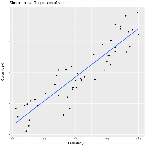
Interpretation: The estimated slope is 1.555, with a p-value of 5.51^{-20}. We reject the null hypothesis, indicating that there is evidence of a significant linear association between x and y.
EJ KORREKTURLÆST
-
Used for Modeling the relationship between one
continuous outcome and two or more predictors (continuous or
categorical).
- Real-world example: Predicting house sale price based on living area, number of bedrooms, and neighborhood quality.
Assumptions * Correct specification: linear
relationship between each predictor and the outcome (additivity).
* Residuals are independent and normally distributed with mean
zero.
* Homoscedasticity: constant variance of residuals for all predictor
values.
* No perfect multicollinearity among predictors.
* No influential outliers unduly affecting the model.
Strengths * Can adjust for multiple confounders or
risk factors simultaneously.
* Provides estimates and inference (CI, p-values) for each predictor’s
unique association with the outcome.
* Basis for variable selection, prediction, and causal modeling in
observational data.
Weaknesses * Sensitive to multicollinearity, which
inflates variances of coefficient estimates.
* Assumes a linear, additive form; interactions or nonlinearity require
extension.
* Outliers and high-leverage points can distort estimates and
inference.
* Interpretation can be complex when including many predictors or
interactions.
Example
-
Null hypothesis (H₀): All regression coefficients
for predictors (β₁, β₂, β₃) are zero (no association).
- Alternative hypothesis (H₁): At least one βᵢ ≠ 0.
R
set.seed(2025)
n <- 100
# Simulate predictors:
living_area     <- runif(n, 800, 3500)        # in square feet
bedrooms        <- sample(2:6, n, replace = TRUE)
neighborhood    <- factor(sample(c("Low","Medium","High"), n, replace = TRUE))
# Simulate price with true model:
price <- 50000 +
         30 * living_area +
         10000 * bedrooms +
         ifelse(neighborhood=="Medium", 20000,
                ifelse(neighborhood=="High", 50000, 0)) +
         rnorm(n, sd = 30000)
df <- data.frame(price, living_area, bedrooms, neighborhood)

# Fit multiple linear regression:
model_mlr <- lm(price ~ living_area + bedrooms + neighborhood, data = df)

# Show model summary:
summary(model_mlr)
OUTPUT
Call:
lm(formula = price ~ living_area + bedrooms + neighborhood, data = df)

Residuals:
   Min     1Q Median     3Q    Max
-76016 -17437   1258  20097  72437

Coefficients:
                     Estimate Std. Error t value Pr(>|t|)
(Intercept)        119719.729  12445.109   9.620 1.07e-15 ***
living_area            26.498      3.685   7.190 1.47e-10 ***
bedrooms             8292.136   2147.637   3.861 0.000206 ***
neighborhoodLow    -59241.209   7084.797  -8.362 5.18e-13 ***
neighborhoodMedium -34072.271   6927.394  -4.918 3.65e-06 ***
---
Signif. codes:  0 '***' 0.001 '**' 0.01 '*' 0.05 '.' 0.1 ' ' 1

Residual standard error: 28490 on 95 degrees of freedom
Multiple R-squared:  0.5891,	Adjusted R-squared:  0.5718
F-statistic: 34.05 on 4 and 95 DF,  p-value: < 2.2e-16
Interpretation:
The overall F-test (in 34.05 on df₁ = 4, df₂ = 95 has p-value = 1.3^{-17}, so reject the null hypothesis.
Individual coefficients: for example, living_area’s estimate is 26.5 (p = 1.47^{-10}), indicating a significant positive association: each additional square foot increases price by about $30 on average.
Similar interpretation applies to bedrooms and neighborhood indicators.
EJ KORREKTURLÆST
-
Used for Assessing the strength and direction of a
linear relationship between two continuous variables.
- Real-world example: Examining whether students’ hours of study correlate with their exam scores.
Assumptions * Observations are independent
pairs.
* Both variables are approximately normally distributed (bivariate
normality).
* Relationship is linear.
* No extreme outliers.
Strengths * Provides both a correlation coefficient
(r) and hypothesis test (t‐statistic, p‐value).
* Confidence interval for the true correlation can be obtained.
* Well understood and widely used.
Weaknesses * Sensitive to outliers, which can
distort r.
* Only measures linear association—will miss non‐linear
relationships.
* Reliant on normality; departures can affect Type I/II error rates.
Example
-
Null hypothesis (H₀): The true Pearson correlation
ρ = 0 (no linear association).
- Alternative hypothesis (H₁): ρ ≠ 0 (a linear association exists).
R
set.seed(2025)
# Simulate data:
n <- 30
hours_studied <- runif(n, min = 0, max = 20)
# Make exam_scores roughly increase with hours_studied + noise:
exam_scores   <- 50 + 2.5 * hours_studied + rnorm(n, sd = 5)

# Perform Pearson correlation test:
pearson_result <- cor.test(hours_studied, exam_scores, method = "pearson")

# Display results:
pearson_result
OUTPUT
	Pearson's product-moment correlation

data:  hours_studied and exam_scores
t = 14.086, df = 28, p-value = 3.108e-14
alternative hypothesis: true correlation is not equal to 0
95 percent confidence interval:
 0.8689058 0.9694448
sample estimates:
      cor
0.9361291
Interpretation: The sample Pearson correlation is 0.936, with t = 14.09 on df = 28 and p-value = 3.11^{-14}. We reject the null hypothesis, indicating that there is evidence of a significant linear association between hours studied and exam scores.
EJ KORREKTURLÆST Used for Assessing the strength and
direction of a monotonic association between two variables using their
ranks.
* Real-world example: Evaluating whether patients’ pain
rankings correlate with their anxiety rankings.
Assumptions * Observations are independent
pairs.
* Variables are at least ordinal.
* The relationship is monotonic (consistently increasing or
decreasing).
Strengths * Nonparametric: does not require
normality of the underlying data.
* Robust to outliers in the original measurements.
* Captures any monotonic relationship, not limited to linear.
Weaknesses * Less powerful than Pearson’s
correlation when the true relationship is linear and data are bivariate
normal.
* Does not distinguish between different monotonic shapes (e.g. concave
vs. convex).
* Tied ranks reduce effective sample size and can complicate exact
p-value calculation.
Example
-
Null hypothesis (H₀): The true Spearman rank
correlation ρ = 0 (no monotonic association).
- Alternative hypothesis (H₁): ρ ≠ 0 (a monotonic association exists).
R
# Simulate two variables with a monotonic relationship:
set.seed(2025)
x <- sample(1:100, 30)                   # e.g., anxiety scores ranked
y <- x + rnorm(30, sd = 15)              # roughly increasing with x, plus noise

# Perform Spearman rank correlation test:
spearman_result <- cor.test(x, y, method = "spearman", exact = FALSE)

# Display results:
spearman_result
OUTPUT
	Spearman's rank correlation rho

data:  x and y
S = 486, p-value = 3.73e-11
alternative hypothesis: true rho is not equal to 0
sample estimates:
      rho
0.8918799
Interpretation: Spearman’s rho = 0.892 with p-value = 3.73^{-11}. We reject the null hypothesis. This indicates that there is evidence of a significant monotonic association between the two variables.
EJ KORREKTURLÆST
-
Used for Assessing the strength and direction of a
monotonic association between two variables based on concordant and
discordant pairs.
- Real-world example: Evaluating whether the ranking of students by homework completion correlates with their ranking by final exam performance.
Assumptions * Observations are independent
pairs.
* Variables are measured on at least an ordinal scale.
* The relationship is monotonic (but not necessarily linear).
Strengths * Nonparametric: does not require any
distributional assumptions.
* Robust to outliers and tied values (with appropriate
corrections).
* Directly interprets probability of concordance vs. discordance.
Weaknesses * Less powerful than Spearman’s rho when
the relationship is strictly monotonic and no ties.
* Tied ranks reduce effective sample size and require tie
corrections.
* Only measures monotonic association, not form or magnitude of
change.
Example
-
Null hypothesis (H₀): Kendall’s τ = 0 (no
association between the two rankings).
- Alternative hypothesis (H₁): τ ≠ 0 (a monotonic association exists).
R
# Simulate two sets of rankings for 25 students:
set.seed(2025)
homework_rank <- sample(1:25, 25)                  # ranking by homework completion
exam_rank     <- homework_rank + rpois(25, lambda=2) - 1  # roughly related with some noise

# Perform Kendall’s tau test:
kendall_result <- cor.test(homework_rank, exam_rank,
                          method  = "kendall",
                          exact   = FALSE)

# Display results:
kendall_result
OUTPUT
	Kendall's rank correlation tau

data:  homework_rank and exam_rank
z = 6.3518, p-value = 2.129e-10
alternative hypothesis: true tau is not equal to 0
sample estimates:
      tau
0.9203643
Interpretation: Kendall’s τ = 0.92 with a two-sided p-value = 2.13^{-10}. We reject the null hypothesis. Thus, there is evidence of a significant monotonic association between homework and exam rankings.
EJ KORREKTURLÆST
-
Used for Modeling the probability of a binary
outcome as a function of two or more predictors.
- Real-world example: Predicting whether a patient has heart disease (yes/no) based on age, cholesterol level, and smoking status.
Assumptions * Outcome is binary (0/1) and
observations are independent.
* Log-odds of the outcome are a linear function of the predictors
(linearity in the logit).
* No perfect multicollinearity among predictors.
* Large enough sample so that maximum likelihood estimates are stable
(rule of thumb: ≥10 events per predictor).
Strengths * Adjusts for multiple confounders
simultaneously.
* Coefficients have clear interpretation as log‐odds (or odds
ratios).
* Flexible: handles continuous, categorical, and interaction terms.
Weaknesses * Sensitive to complete or quasi‐complete
separation (can prevent convergence).
* Assumes linearity in the logit—requires transformation or splines if
violated.
* Interpretation of interactions and higher‐order terms can be
complex.
* Requires adequate sample size, especially when events are rare.
Example
-
Null hypothesis (H₀): All predictor coefficients β₁
= β₂ = β₃ = 0 (none of the variables affect disease odds).
- Alternative hypothesis (H₁): At least one βᵢ ≠ 0 (at least one predictor affects odds).
R
set.seed(2025)
n <- 200
# Simulate predictors:
age          <- rnorm(n, mean = 60, sd = 10)
cholesterol  <- rnorm(n, mean = 200, sd = 30)
smoker       <- factor(rbinom(n, 1, 0.3), labels = c("No", "Yes"))

# Simulate binary outcome via logistic model:
logit_p <- -5 + 0.04 * age + 0.01 * cholesterol + 1.2 * (smoker=="Yes")
p        <- 1 / (1 + exp(-logit_p))
disease  <- rbinom(n, 1, p)

df <- data.frame(disease = factor(disease, labels = c("No","Yes")),
                 age, cholesterol, smoker)

# Fit multiple logistic regression:
model <- glm(disease ~ age + cholesterol + smoker,
             data = df,
             family = binomial)

# Show summary and odds ratios:
summary(model)
OUTPUT
Call:
glm(formula = disease ~ age + cholesterol + smoker, family = binomial,
    data = df)

Coefficients:
             Estimate Std. Error z value Pr(>|z|)
(Intercept) -7.016100   1.712922  -4.096 4.20e-05 ***
age          0.075418   0.017734   4.253 2.11e-05 ***
cholesterol  0.008465   0.005440   1.556  0.11971
smokerYes    0.998927   0.360721   2.769  0.00562 **
---
Signif. codes:  0 '***' 0.001 '**' 0.01 '*' 0.05 '.' 0.1 ' ' 1

(Dispersion parameter for binomial family taken to be 1)

    Null deviance: 265.63  on 199  degrees of freedom
Residual deviance: 237.72  on 196  degrees of freedom
AIC: 245.72

Number of Fisher Scoring iterations: 3
R
exp(coef(model))
OUTPUT
(Intercept)         age cholesterol   smokerYes
0.000897318 1.078334765 1.008500725 2.715367476
R
exp(confint(model))
OUTPUT
Waiting for profiling to be done...OUTPUT
                   2.5 %     97.5 %
(Intercept) 2.650867e-05 0.02260073
age         1.042852e+00 1.11825331
cholesterol 9.979236e-01 1.01955252
smokerYes   1.347682e+00 5.57661867
Interpretation:
The Wald test for each coefficient (from summary(model)) gives a z-statistic and p-value. For example, if the coefficient for age is β̂ = 0.04 (p = 0.01), its odds ratio is exp(0.04) ≈ 1.04 (95% CI from exp(confint(model))), meaning each additional year of age multiplies the odds of disease by about 1.04.
A significant p-value (e.g., p < 0.05) for cholesterol indicates that higher cholesterol is associated with increased odds (OR = exp(β̂_cholesterol)).
A significant positive coefficient for smoker (β̂ ≈ 1.2, OR ≈ 3.3) implies smokers have about 3.3 times the odds of disease compared to non-smokers, adjusting for age and cholesterol.
You would reject the null hypothesis overall, concluding that at least one predictor is significantly associated with the outcome.
EJ KORREKTURLÆST
-
Used for Modeling count data (events per unit time
or space) as a function of one or more predictors.
- Real-world example: Predicting the number of daily emergency room visits based on average daily temperature.
Assumptions * Counts follow a Poisson distribution
(mean = variance).
* Events occur independently.
* The log of the expected count is a linear function of the
predictors.
* No excessive zero‐inflation (if present, consider zero‐inflated
models).
Strengths * Naturally handles non‐negative integer
outcomes.
* Estimates incidence rate ratios (IRRs) that are easy to
interpret.
* Can include both categorical and continuous predictors.
Weaknesses * Sensitive to overdispersion (variance
> mean); may need quasi‐Poisson or negative binomial.
* Assumes log‐linear relationship—misspecification leads to bias.
* Influential observations (e.g., days with extreme counts) can distort
estimates.
Example
-
Null hypothesis (H₀): Temperature has no effect on
the expected number of ER visits (β₁ = 0).
- Alternative hypothesis (H₁): Temperature affects the expected number of ER visits (β₁ ≠ 0).
R
set.seed(2025)
# Simulate 100 days of data:
n_days      <- 100
temp        <- runif(n_days, min = 0,  max = 30)              # average daily temperature (°C)
# True model: log(rate) = 1 + 0.05 * temp
log_rate    <- 1 + 0.05 * temp
expected    <- exp(log_rate)
er_visits   <- rpois(n_days, lambda = expected)              # simulated counts

df <- data.frame(er_visits, temp)

# Fit Poisson regression:
pois_fit <- glm(er_visits ~ temp, family = poisson(link = "log"), data = df)

# Display summary:
summary(pois_fit)
OUTPUT
Call:
glm(formula = er_visits ~ temp, family = poisson(link = "log"),
    data = df)

Coefficients:
            Estimate Std. Error z value Pr(>|z|)
(Intercept) 0.982531   0.101027   9.725   <2e-16 ***
temp        0.052793   0.004823  10.945   <2e-16 ***
---
Signif. codes:  0 '***' 0.001 '**' 0.01 '*' 0.05 '.' 0.1 ' ' 1

(Dispersion parameter for poisson family taken to be 1)

    Null deviance: 233.15  on 99  degrees of freedom
Residual deviance: 104.41  on 98  degrees of freedom
AIC: 463.81

Number of Fisher Scoring iterations: 4
Interpretation: The estimated coefficient for temperature is 0.053, giving an incidence rate ratio IRR = 1.054. With a p-value = 7.01^{-28}, we reject the null hypothesis. This means each 1 °C increase in average daily temperature is associated with a multiplicative change of approximately 1.054 in the expected number of ER visits.
EJ KORREKTURLÆST
-
Used for Modeling overdispersed count data
(variance > mean) as a function of one or more predictors.
- Real-world example: Predicting the number of daily asthma attacks per patient based on air pollution level when counts show extra-Poisson variation.
Assumptions * Counts follow a negative binomial
distribution (allows variance > mean).
* Events occur independently.
* The log of the expected count is a linear function of the
predictors.
* Overdispersion parameter is constant across observations.
Strengths * Handles overdispersion naturally without
biasing standard errors.
* Estimates incidence rate ratios (IRRs) with correct inference.
* Can include both continuous and categorical predictors.
Weaknesses * Requires estimation of an extra
dispersion parameter, which may be unstable in small samples.
* Sensitive to model misspecification (link function, omitted
covariates).
* Influential observations can still distort estimates if extreme.
Example
-
Null hypothesis (H₀): Air pollution level has no
effect on the expected number of asthma attacks (β₁ = 0).
- Alternative hypothesis (H₁): Air pollution level affects the expected number of asthma attacks (β₁ ≠ 0).
R
# install.packages("MASS")  # if necessary
library(MASS)

set.seed(2025)
n_patients <- 150
# Simulate predictor: average daily PM2.5 level (µg/m³)
pm25       <- runif(n_patients, min = 5, max = 50)
# True model: log(µ) = 0.5 + 0.04 * pm25, dispersion theta = 2
log_mu     <- 0.5 + 0.04 * pm25
mu         <- exp(log_mu)
attacks    <- rnbinom(n_patients, mu = mu, size = 2)

df_nb <- data.frame(attacks, pm25)

# Fit negative binomial regression:
nb_fit <- glm.nb(attacks ~ pm25, data = df_nb)

# Display summary:
summary(nb_fit)
OUTPUT
Call:
glm.nb(formula = attacks ~ pm25, data = df_nb, init.theta = 2.392967844,
    link = log)

Coefficients:
            Estimate Std. Error z value Pr(>|z|)
(Intercept) 0.418832   0.170421   2.458    0.014 *
pm25        0.045102   0.005085   8.869   <2e-16 ***
---
Signif. codes:  0 '***' 0.001 '**' 0.01 '*' 0.05 '.' 0.1 ' ' 1

(Dispersion parameter for Negative Binomial(2.393) family taken to be 1)

    Null deviance: 250.51  on 149  degrees of freedom
Residual deviance: 167.61  on 148  degrees of freedom
AIC: 823.46

Number of Fisher Scoring iterations: 1

              Theta:  2.393
          Std. Err.:  0.410

 2 x log-likelihood:  -817.455
Interpretation: The estimated coefficient for PM2.5 is 0.045, giving an incidence rate ratio IRR = 1.046. With p-value = 7.38^{-19}, we reject the null hypothesis. This means each 1 µg/m³ increase in PM2.5 is associated with a multiplicative change of approximately 1.046 in the expected number of asthma attacks, accounting for overdispersion.
EJ KORREKTURLÆST
Used for * Modeling an ordinal outcome (with more
than two ordered categories) as a function of one or more
predictors.
* Real-world example: Predicting customer satisfaction
levels (Low, Medium, High) based on service wait time and price.
Assumptions * The dependent variable is ordinal with
a meaningful order.
* Proportional odds (parallel lines): the effect of
each predictor is the same across all thresholds between outcome
categories.
* Observations are independent.
* No multicollinearity among predictors.
Strengths * Makes efficient use of the ordering
information in the outcome.
* Provides interpretable odds‐ratios for cumulative probabilities.
* More powerful than nominal models (e.g., multinomial logit) when the
order matters.
Weaknesses * Relies on the proportional‐odds
assumption; violation can bias estimates.
* Interpretation can be less intuitive than linear regression.
* Cannot easily accommodate non‐proportional effects without
extension.
Example
-
Null hypothesis (H₀): Waiting time has no effect on
the odds of higher satisfaction (\(\beta_{\text{wait}} = 0\)).
- Alternative hypothesis (H₁): Waiting time affects the odds of higher satisfaction (\(\beta_{\text{wait}} \neq 0\)).
R
# Load data and package
library(MASS)

set.seed(2025)
n <- 120
# Simulate predictors:
wait_time <- runif(n,  5, 60)      # waiting time in minutes
price     <- runif(n, 10, 100)     # price in dollars

# Simulate an ordinal outcome via latent variable:
latent   <- 2 - 0.03 * wait_time - 0.01 * price + rnorm(n)
# Define thresholds for three satisfaction levels:
# latent ≤ 0: Low; 0 < latent ≤ 1: Medium; latent > 1: High
satisfaction <- cut(latent,
                    breaks = c(-Inf, 0, 1, Inf),
                    labels = c("Low","Medium","High"),
                    ordered_result = TRUE)

df <- data.frame(satisfaction, wait_time, price)

# Fit proportional‐odds (ordinal logistic) model:
model_polr <- polr(satisfaction ~ wait_time + price, data = df, Hess = TRUE)

# Summarize coefficients and compute p‐values:
ctable <- coef(summary(model_polr))
pvals  <- pnorm(abs(ctable[,"t value"]), lower.tail = FALSE) * 2
results <- cbind(ctable, "p value" = round(pvals, 3))

# Display thresholds and predictor effects:
results
OUTPUT
                  Value  Std. Error   t value p value
wait_time   -0.04036665 0.011844352 -3.408093   0.001
price       -0.02267858 0.006578292 -3.447488   0.001
Low|Medium  -3.34230915 0.625031561 -5.347425   0.000
Medium|High -1.78229869 0.564771833 -3.155785   0.002
Interpretation: The estimated coefficient for wait_time is -0.04.
The odds‐ratio is 0.96, meaning each additional minute of wait changes the odds of being in a higher satisfaction category by that factor.
A p‐value of 0.001 for wait_time indicates rejecting H₀: wait time significantly affects satisfaction odds.
Similar interpretation applies to price.
EJ KORREKTURLÆST * Used for Modeling continuous
outcomes with both fixed effects (predictors of interest) and random
effects (to account for grouped or repeated measures).
* Real-world example: Evaluating the effect of a new
teaching method on student test scores, while accounting for variability
between classrooms and schools.
Assumptions * Linear relationship between predictors
and outcome.
* Residuals are independent and normally distributed with mean
zero.
* Random effects are normally distributed.
* Homoscedasticity: constant variance of residuals.
* Random effects structure correctly specified (e.g., intercepts and/or
slopes).
Strengths * Accounts for correlation within clusters
(e.g., pupils within the same classroom).
* Can handle unbalanced data and missing observations within
clusters.
* Flexibly models complex hierarchical or longitudinal data
structures.
Weaknesses * Model specification (random effects
structure) can be challenging.
* Parameter estimation can be computationally intensive and may fail to
converge.
* Inference (p-values) often relies on approximations or additional
packages.
Example * Null hypothesis (H₀): The
new teaching method has no effect on student test scores (fixed effect
β_method = 0).
* Alternative hypothesis (H₁): The new teaching method
affects student test scores (β_method ≠ 0).
R
# Install/load necessary packages
# install.packages("lme4"); install.packages("lmerTest")
library(lme4)
OUTPUT
Loading required package: MatrixOUTPUT
Registered S3 method overwritten by 'lme4':
  method           from
  na.action.merMod car
R
library(lmerTest)
OUTPUT
Attaching package: 'lmerTest'OUTPUT
The following object is masked from 'package:lme4':

    lmer
OUTPUT
The following object is masked from 'package:stats':

    step
R
set.seed(2025)
# Simulate data: 100 students in 10 classrooms within 3 schools
n_schools   <-  3
n_classes   <- 10
students_pc <- 10

school      <- factor(rep(1:n_schools, each = n_classes * students_pc))
class       <- factor(rep(1:(n_schools * n_classes), each = students_pc))
method      <- factor(rep(rep(c("Control","NewMethod"), each = students_pc/2), times = n_schools * n_classes))
# True model: intercept = 70, method effect = 5 points, random intercepts for class & school, residual sd = 8
score <- 70 +
         ifelse(method=="NewMethod", 5, 0) +
         rnorm(n_schools * n_classes * students_pc, sd = 8) +
         rep(rnorm(n_schools * n_classes, sd = 4), each = students_pc) +
         rep(rnorm(n_schools,            sd = 6), each = n_classes * students_pc)

df <- data.frame(score, method, class, school)

# Fit linear mixed-effects model with random intercepts for school and class:
lme_fit <- lmer(score ~ method + (1 | school/class), data = df)

# Summarize model (includes p-values via lmerTest):
summary(lme_fit)
OUTPUT
Linear mixed model fit by REML. t-tests use Satterthwaite's method [
lmerModLmerTest]
Formula: score ~ method + (1 | school/class)
   Data: df

REML criterion at convergence: 2132.4

Scaled residuals:
     Min       1Q   Median       3Q      Max
-2.69138 -0.67244  0.04868  0.66053  2.86344

Random effects:
 Groups       Name        Variance Std.Dev.
 class:school (Intercept) 20.88    4.570
 school       (Intercept) 91.42    9.561
 Residual                 61.31    7.830
Number of obs: 300, groups:  class:school, 30; school, 3

Fixed effects:
                Estimate Std. Error       df t value Pr(>|t|)
(Intercept)      64.6076     5.6194   2.0276  11.497  0.00712 **
methodNewMethod   5.9555     0.9042 268.9993   6.587 2.35e-10 ***
---
Signif. codes:  0 '***' 0.001 '**' 0.01 '*' 0.05 '.' 0.1 ' ' 1

Correlation of Fixed Effects:
            (Intr)
methdNwMthd -0.080
Interpretation: The fixed-effect estimate for NewMethod is 5.96 points (SE = 0.9), with p = 2.35^{-10}. We reject the null hypothesis. Thus, there is evidence that the new teaching method significantly changes test scores, accounting for classroom and school variability.
EJ KORREKTURLÆST
-
Used for Modeling non-normal outcomes (e.g. binary,
counts) with both fixed effects and random effects.
- Real-world example: Predicting whether patients are readmitted (yes/no) based on age and comorbidity score, with random intercepts for each hospital.
Assumptions * Observations within each cluster
(e.g. hospital) are correlated, but clusters are independent.
* The conditional distribution of the outcome given predictors and
random effects follows a specified exponential‐family distribution
(e.g. binomial, Poisson).
* The link function (e.g. logit, log) correctly relates the linear
predictor to the mean of the outcome.
* Random effects are normally distributed.
Strengths * Can accommodate hierarchical or
longitudinal data and non-Gaussian outcomes.
* Estimates both population‐level (fixed) effects and cluster‐specific
(random) variation.
* Flexible: supports a variety of link functions and distributions.
Weaknesses * Computationally intensive; convergence
can fail with complex random‐effects structures.
* Inference (especially p-values for fixed effects) relies on
approximations.
* Model specification (random slopes, link choice) can be
challenging.
Example
-
Null hypothesis (H₀): The log-odds of readmission
do not depend on age (β_age = 0).
- Alternative hypothesis (H₁): Age affects the log-odds of readmission (β_age ≠ 0).
R
# Load packages
library(lme4)

set.seed(2025)
# Simulate data for 2000 patients in 20 hospitals:
n_hospitals <- 20
patients_per <- 100
hospital   <- factor(rep(1:n_hospitals, each = patients_per))
age        <- rnorm(n_hospitals * patients_per, mean = 65, sd = 10)
comorbidity<- rpois(n_hospitals * patients_per, lambda = 2)

# True model: logit(p) = -2 + 0.03*age + 0.5*comorbidity + random intercept by hospital
logit_p    <- -2 + 0.03 * age + 0.5 * comorbidity + rnorm(n_hospitals, 0, 0.5)[hospital]
p_readmit  <- plogis(logit_p)
readmit    <- rbinom(n_hospitals * patients_per, size = 1, prob = p_readmit)

df_glmm <- data.frame(readmit = factor(readmit, levels = c(0,1)),
                      age, comorbidity, hospital)

# Fit a binomial GLMM with random intercepts for hospital:
glmm_fit <- glmer(readmit ~ age + comorbidity + (1 | hospital),
                  data = df_glmm, family = binomial(link = "logit"))

# Display summary:
summary(glmm_fit)
OUTPUT
Generalized linear mixed model fit by maximum likelihood (Laplace
  Approximation) [glmerMod]
 Family: binomial  ( logit )
Formula: readmit ~ age + comorbidity + (1 | hospital)
   Data: df_glmm

      AIC       BIC    logLik -2*log(L)  df.resid
   2200.4    2222.8   -1096.2    2192.4      1996

Scaled residuals:
    Min      1Q  Median      3Q     Max
-3.9499 -0.9147  0.4555  0.6420  1.7336

Random effects:
 Groups   Name        Variance Std.Dev.
 hospital (Intercept) 0.1931   0.4395
Number of obs: 2000, groups:  hospital, 20

Fixed effects:
             Estimate Std. Error z value Pr(>|z|)
(Intercept) -2.132901   0.370427  -5.758 8.51e-09 ***
age          0.035056   0.005317   6.593 4.30e-11 ***
comorbidity  0.457562   0.044238  10.343  < 2e-16 ***
---
Signif. codes:  0 '***' 0.001 '**' 0.01 '*' 0.05 '.' 0.1 ' ' 1

Correlation of Fixed Effects:
            (Intr) age
age         -0.932
comorbidity -0.293  0.101
Interpretation: The fixed‐effect estimate for age is 0.035 (SE = 0.005), giving an odds ratio of 1.036 per year of age. With a z‐value = 6.59 and p ≈ 4.3^{-11}, we reject the null hypothesis. This indicates that age is significantly associated with higher odds of readmission, accounting for hospital clustering.
EJ KORREKTURLÆST
-
Used for Modeling correlated or clustered data
(e.g., repeated measures, longitudinal, or clustered observations) when
interest lies in population‐averaged effects rather than
subject‐specific effects.
- Real-world example: Estimating the effect of a diabetes education program on the probability of glycemic control (A1C < 7%) over multiple clinic visits per patient.
Assumptions * Clustered or repeated observations per
subject/cluster with some “working” correlation structure (e.g.,
exchangeable, autoregressive).
* Correct specification of the link function and the mean model (e.g.,
logit link for binary outcomes).
* Missing data are missing completely at random (MCAR) or missing at
random (MAR), assuming missingness only depends on observed
covariates.
* Large‐sample inference: GEE relies on asymptotic properties (number of
clusters ≫ 1).
Strengths * Robust (“sandwich”) standard errors even
if the working correlation structure is mis‐specified.
* Provides marginal (population‐averaged) estimates, often of direct
interest in public health/epidemiology.
* Accommodates a variety of outcomes (binary, count, continuous) via
appropriate link and family.
Weaknesses * Efficiency can be lost if the working
correlation is far from the truth (though estimates remain
consistent).
* Inference is asymptotic—small numbers of clusters can lead to biased
standard errors.
* Does not model subject‐specific trajectories; cannot estimate
random‐effects variance components.
Example
-
Null hypothesis (H₀): The education program has no
effect on odds of glycemic control over time (β_edu = 0).
- Alternative hypothesis (H₁): The education program changes the odds of glycemic control over time (β_edu ≠ 0).
R
# Install/load necessary package:
# install.packages("geepack")
library(geepack)

set.seed(2025)
# Simulate data: 100 patients (clusters), each with 4 visits
n_patients   <- 100
visits_per   <- 4
patient_id   <- rep(1:n_patients, each = visits_per)
visit_number <- rep(1:visits_per, times = n_patients)

# Simulate a binary program indicator (0=no program, 1=received education), randomly assigned at baseline
edu_program  <- rbinom(n_patients, 1, 0.5)
edu          <- rep(edu_program, each = visits_per)

# Simulate time effect (visits 1–4 coded 0–3) and baseline covariate (e.g., age)
age_cont     <- rnorm(n_patients, mean = 60, sd = 10)
age          <- rep(age_cont, each = visits_per)

# True population‐averaged logistic model:
# logit(p_ij) = -1 + 0.4 * edu_i - 0.02 * age_i + 0.3 * visit_number_j
# For simplicity, ignore cluster‐specific random effect; correlation introduced via GEE working structure.
lin_pred     <- -1 +
                0.4 * edu +
               -0.02 * age +
                0.3 * visit_number
prob         <- plogis(lin_pred)

# Simulate binary outcome: glycemic control (1=yes, 0=no)
gly_control  <- rbinom(n_patients * visits_per, 1, prob)

df_gee <- data.frame(
  patient_id   = factor(patient_id),
  visit_number = visit_number,
  edu          = factor(edu, labels = c("NoEdu","Edu")),
  age          = age,
  gly_control  = gly_control
)

# Fit GEE with exchangeable working correlation:
gee_fit <- geeglm(
  gly_control ~ edu + age + visit_number,
  id            = patient_id,
  family        = binomial(link = "logit"),
  corstr        = "exchangeable",
  data          = df_gee
)

# Display summary:
summary(gee_fit)
OUTPUT
Call:
geeglm(formula = gly_control ~ edu + age + visit_number, family = binomial(link = "logit"),
    data = df_gee, id = patient_id, corstr = "exchangeable")

 Coefficients:
             Estimate  Std.err   Wald Pr(>|W|)
(Intercept)  -1.84098  0.87073  4.470   0.0345 *
eduEdu        0.55189  0.24796  4.954   0.0260 *
age          -0.01791  0.01287  1.934   0.1643
visit_number  0.55376  0.10903 25.795  3.8e-07 ***
---
Signif. codes:  0 '***' 0.001 '**' 0.01 '*' 0.05 '.' 0.1 ' ' 1

Correlation structure = exchangeable
Estimated Scale Parameters:

            Estimate Std.err
(Intercept)   0.9761  0.1171
  Link = identity

Estimated Correlation Parameters:
      Estimate Std.err
alpha  0.00166 0.03069
Number of clusters:   100  Maximum cluster size: 4
**Interpretation:*’
The estimated coefficient for edu (Edu vs. NoEdu) is 0.552 . Its robust (“sandwich”) standard error is 0.248
, yielding a Wald‐type z = 2.23, with p = 0.026. We reject the null hypothesis. This indicates that, across all visits and patients, those in the education program have significantly difference in odds of glycemic control compared to those without education.
The coefficient for age equals -0.0179 (p = 0.164), indicating each additional year of age multiplies the odds of control by exp(-0.0179).
The visit_number effect is 0.554 per visit (p = 3.8^{-7}), showing whether odds of control change over successive visits.
Because GEE uses a sandwich estimator, these inferences remain valid even if “exchangeable” correlation is not exactly correct, provided we have a sufficiently large number of patients.
Kontingenstabel- og proportions-tests
EJ KORREKTURLÆST
-
Used for Testing whether the proportions of paired
binary outcomes differ (i.e., detecting marginal changes in a 2×2 paired
table).
- Real-world example: Determining if a new diagnostic test classification (Positive/Negative) differs from an existing “gold standard” classification on the same patients.
Assumptions * Data consist of paired binary
observations (e.g., before/after, test1/test2) on the same
subjects.
* Discordant cell counts (subjects where Test A=Positive & Test
B=Negative or vice versa) are sufficiently large (≥ 10) for the χ²
approximation; otherwise use exact McNemar.
* Each pair is independent of all other pairs.
Strengths * Simple to implement for paired binary
data.
* Specifically tests for a change in proportion rather than overall
association.
* Does not require marginal homogeneity for concordant pairs (only
discordant pairs matter).
Weaknesses * Ignores concordant pairs (those where
both methods agree), focusing only on discordant counts.
* χ² approximation can be invalid if discordant counts are
small—requires exact test.
* Only applicable to 2×2 paired tables (binary outcomes).
Example
-
Null hypothesis (H₀): The probability of discordant
outcomes is the same in both directions (b = c).
- Alternative hypothesis (H₁): The probability of discordant outcomes differs (b ≠ c).
R
# Simulated paired binary data: OldTest vs. NewTest (n = 100 patients)
#      NewTest
# OldTest  Positive  Negative
# Positive      30        20   (b = 20)
# Negative      10        40   (c = 10)

ctab <- matrix(c(30, 20,
                 10, 40),
               nrow = 2,
               byrow = TRUE,
               dimnames = list(
                 OldTest = c("Positive","Negative"),
                 NewTest = c("Positive","Negative")
               ))

# Perform McNemar’s test (χ² approximation):
mcnemar_result <- mcnemar.test(ctab, correct = FALSE)

# Display results:
mcnemar_result
OUTPUT
	McNemar's Chi-squared test

data:  ctab
McNemar's chi-squared = 3.3, df = 1, p-value = 0.07
Interpretation: The McNemar χ² statistic is 3.33 with p-value = 0.0679. We fail to reject the null hypothesis. Since b (OldTest Positive, NewTest Negative) = 20 and c (OldTest Negative, NewTest Positive) = 10, a significant result would indicate that the switch in classifications is not symmetric—i.e., the new test’s positive/negative calls differ from the old test more often in one direction than the other.
EJ KORREKTURLÆST
-
Used for Testing independence between two
categorical variables in a small-sample 2×2 contingency table.
- Real-world example: Examining whether a new antibiotic leads to cure versus failure in 15 patients (small sample where χ² might be invalid).
Assumptions * Observations are independent.
* Data form a 2×2 table (binary outcome × binary exposure).
* Marginal totals are fixed (conditional inference on margins).
Strengths * Exact p-value without relying on
large-sample approximations.
* Valid even when expected cell counts are very small or zero.
* Simple to implement in R via fisher.test().
Weaknesses * Only directly applies to 2×2 tables;
extensions to larger tables exist but are computationally
intensive.
* Does not provide an effect-size estimate beyond the odds ratio (which
must be computed separately).
* Can be conservative (lower power) compared to asymptotic tests with
moderate sample sizes.
Example
-
Null hypothesis (H₀): Treatment and outcome are
independent (odds ratio = 1).
- Alternative hypothesis (H₁): Treatment and outcome are not independent (odds ratio ≠ 1).
R
# Construct a 2×2 contingency table:
#               Outcome
# Treatment   Cure  Failure
#   New        7      3
#   Standard   2      3

ctab <- matrix(c(7, 3,
                 2, 3),
               nrow = 2,
               byrow = TRUE,
               dimnames = list(
                 Treatment = c("New", "Standard"),
                 Outcome   = c("Cure", "Failure")
               ))

# Perform Fisher’s exact test:
fisher_result <- fisher.test(ctab, alternative = "two.sided")

# Display results:
fisher_result
OUTPUT
	Fisher's Exact Test for Count Data

data:  ctab
p-value = 0.3
alternative hypothesis: true odds ratio is not equal to 1
95 percent confidence interval:
  0.2329 59.0957
sample estimates:
odds ratio
     3.196
Interpretation: Fisher’s exact test yields an odds ratio estimate of 3.2 with a two-sided p-value = 0.329. We fail to reject the null hypothesis. Thus, there is no evidence of a difference in cure rates between the two treatments.
EJ KORREKTURLÆST VÆR SÆRLIGT OPMÆRKSOM HER - DER VAR STORE UDFORDRINGER…
-
Used for Testing independence in a 2×2 contingency
table via an unconditional exact test.
- Real-world example: Determining if a new pain medication and placebo differ in adverse event rates when sample sizes are small.
Assumptions * Observations are independent and each
subject contributes exactly one cell in the 2×2 table.
* Only one margin (row or column totals) is fixed; the other margin is
free.
* Binary outcome (e.g., “Adverse Event: Yes/No”) and binary grouping
(“Medication vs. Placebo”).
Strengths * More powerful than Fisher’s exact test
because it does not condition on both margins.
* Provides an exact p-value without relying on large‐sample
approximations.
* Particularly advantageous when margins are not fixed by design.
Weaknesses * Computationally slower than Fisher’s
exact test for larger sample sizes.
* Only applies to 2×2 tables (binary × binary).
* Requires installation of the Barnard package (not in
base R).
Example
-
Null hypothesis (H₀): The probability of an adverse
event is the same in the Medication and Placebo groups (no
association).
- Alternative hypothesis (H₁): The probability of an adverse event differs between Medication and Placebo.
R
# Install and load the Barnard package (only once if not already installed):
# install.packages("Barnard")
library(Barnard)

# Define the 2×2 counts:
#              AdverseEvent
# Treatment   Yes   No
#   Medication  2     8
#   Placebo     7     3
n1 <- 2   # Medication & Yes
n2 <- 8   # Medication & No
n3 <- 7   # Placebo    & Yes
n4 <- 3   # Placebo    & No

# Run Barnard's unconditional exact test:
barnard_result <- barnard.test(n1, n2, n3, n4, pooled = TRUE)
OUTPUT
Barnard's Unconditional Test

           Treatment I Treatment II
Outcome I            2            8
Outcome II           7            3

Null hypothesis: Treatments have no effect on the outcomes
Score statistic = 2.24733
Nuisance parameter = 0.666 (One sided), 0.5 (Two sided)
P-value = 0.0167869 (One sided), 0.0334587 (Two sided)
R
# Display the test result:
barnard_result
OUTPUT
$statistic.table
       n1 n2 statistic include.in.p.value
  [1,]  0  1   0.92803                  0
  [2,]  0  2   1.34840                  0
  [3,]  0  3   1.69932                  0
  [4,]  0  4   2.02260                  0
  [5,]  0  5   2.33550                  1
  [6,]  0  6   2.64820                  1
  [7,]  0  7   2.96836                  1
  [8,]  0  8   3.30289                  1
  [9,]  0  9   3.65902                  1
 [10,]  0 10   4.04520                  1
 [11,]  0 11   4.47214                  1
 [12,]  1  0  -1.13426                  0
 [13,]  1  1  -0.14982                  0
 [14,]  1  2   0.44057                  0
 [15,]  1  3   0.89893                  0
 [16,]  1  4   1.29750                  0
 [17,]  1  5   1.66739                  0
 [18,]  1  6   2.02603                  0
 [19,]  1  7   2.38542                  1
 [20,]  1  8   2.75556                  1
 [21,]  1  9   3.14627                  1
 [22,]  1 10   3.56867                  1
 [23,]  1 11   4.03687                  1
 [24,]  2  0  -1.64804                  0
 [25,]  2  1  -0.81819                  0
 [26,]  2  2  -0.22473                  0
 [27,]  2  3   0.25950                  0
 [28,]  2  4   0.68657                  0
 [29,]  2  5   1.08369                  0
 [30,]  2  6   1.46795                  0
 [31,]  2  7   1.85210                  0
 [32,]  2  8   2.24733                  1
 [33,]  2  9   2.66521                  1
 [34,]  2 10   3.11940                  1
 [35,]  2 11   3.62800                  1
 [36,]  3  0  -2.07695                  0
 [37,]  3  1  -1.34840                  0
 [38,]  3  2  -0.77850                  0
 [39,]  3  3  -0.29424                  0
 [40,]  3  4   0.14135                  0
 [41,]  3  5   0.55048                  0
 [42,]  3  6   0.94863                  0
 [43,]  3  7   1.34840                  0
 [44,]  3  8   1.76175                  0
 [45,]  3  9   2.20193                  0
 [46,]  3 10   2.68566                  1
 [47,]  3 11   3.23669                  1
 [48,]  4  0  -2.47207                  2
 [49,]  4  1  -1.81650                  0
 [50,]  4  2  -1.27506                  0
 [51,]  4  3  -0.80099                  0
 [52,]  4  4  -0.36699                  0
 [53,]  4  5   0.04517                  0
 [54,]  4  6   0.44947                  0
 [55,]  4  7   0.85829                  0
 [56,]  4  8   1.28446                  0
 [57,]  4  9   1.74333                  0
 [58,]  4 10   2.25588                  1
 [59,]  4 11   2.85450                  1
 [60,]  5  0  -2.85450                  2
 [61,]  5  1  -2.25588                  2
 [62,]  5  2  -1.74333                  0
 [63,]  5  3  -1.28446                  0
 [64,]  5  4  -0.85829                  0
 [65,]  5  5  -0.44947                  0
 [66,]  5  6  -0.04517                  0
 [67,]  5  7   0.36699                  0
 [68,]  5  8   0.80099                  0
 [69,]  5  9   1.27506                  0
 [70,]  5 10   1.81650                  0
 [71,]  5 11   2.47207                  1
 [72,]  6  0  -3.23669                  2
 [73,]  6  1  -2.68566                  2
 [74,]  6  2  -2.20193                  0
 [75,]  6  3  -1.76175                  0
 [76,]  6  4  -1.34840                  0
 [77,]  6  5  -0.94863                  0
 [78,]  6  6  -0.55048                  0
 [79,]  6  7  -0.14135                  0
 [80,]  6  8   0.29424                  0
 [81,]  6  9   0.77850                  0
 [82,]  6 10   1.34840                  0
 [83,]  6 11   2.07695                  0
 [84,]  7  0  -3.62800                  2
 [85,]  7  1  -3.11940                  2
 [86,]  7  2  -2.66521                  2
 [87,]  7  3  -2.24733                  2
 [88,]  7  4  -1.85210                  0
 [89,]  7  5  -1.46795                  0
 [90,]  7  6  -1.08369                  0
 [91,]  7  7  -0.68657                  0
 [92,]  7  8  -0.25950                  0
 [93,]  7  9   0.22473                  0
 [94,]  7 10   0.81819                  0
 [95,]  7 11   1.64804                  0
 [96,]  8  0  -4.03687                  2
 [97,]  8  1  -3.56867                  2
 [98,]  8  2  -3.14627                  2
 [99,]  8  3  -2.75556                  2
[100,]  8  4  -2.38542                  2
[101,]  8  5  -2.02603                  0
[102,]  8  6  -1.66739                  0
[103,]  8  7  -1.29750                  0
[104,]  8  8  -0.89893                  0
[105,]  8  9  -0.44057                  0
[106,]  8 10   0.14982                  0
[107,]  8 11   1.13426                  0
[108,]  9  0  -4.47214                  2
[109,]  9  1  -4.04520                  2
[110,]  9  2  -3.65902                  2
[111,]  9  3  -3.30289                  2
[112,]  9  4  -2.96836                  2
[113,]  9  5  -2.64820                  2
[114,]  9  6  -2.33550                  2
[115,]  9  7  -2.02260                  0
[116,]  9  8  -1.69932                  0
[117,]  9  9  -1.34840                  0
[118,]  9 10  -0.92803                  0

$nuisance.matrix
         [,1]      [,2]      [,3]
   [1,] 0.000 0.000e+00 0.000e+00
   [2,] 0.001 4.556e-13 1.246e-10
   [3,] 0.002 1.438e-11 1.971e-09
   [4,] 0.003 1.076e-10 9.865e-09
   [5,] 0.004 4.473e-10 3.083e-08
   [6,] 0.005 1.346e-09 7.441e-08
   [7,] 0.006 3.302e-09 1.526e-07
   [8,] 0.007 7.038e-09 2.795e-07
   [9,] 0.008 1.353e-08 4.714e-07
  [10,] 0.009 2.404e-08 7.466e-07
  [11,] 0.010 4.014e-08 1.125e-06
  [12,] 0.011 6.374e-08 1.629e-06
  [13,] 0.012 9.709e-08 2.281e-06
  [14,] 0.013 1.428e-07 3.106e-06
  [15,] 0.014 2.040e-07 4.131e-06
  [16,] 0.015 2.840e-07 5.383e-06
  [17,] 0.016 3.866e-07 6.890e-06
  [18,] 0.017 5.161e-07 8.681e-06
  [19,] 0.018 6.772e-07 1.079e-05
  [20,] 0.019 8.748e-07 1.324e-05
  [21,] 0.020 1.115e-06 1.608e-05
  [22,] 0.021 1.402e-06 1.932e-05
  [23,] 0.022 1.745e-06 2.301e-05
  [24,] 0.023 2.148e-06 2.718e-05
  [25,] 0.024 2.620e-06 3.186e-05
  [26,] 0.025 3.167e-06 3.709e-05
  [27,] 0.026 3.798e-06 4.290e-05
  [28,] 0.027 4.522e-06 4.933e-05
  [29,] 0.028 5.347e-06 5.641e-05
  [30,] 0.029 6.281e-06 6.418e-05
  [31,] 0.030 7.335e-06 7.268e-05
  [32,] 0.031 8.519e-06 8.193e-05
  [33,] 0.032 9.842e-06 9.198e-05
  [34,] 0.033 1.131e-05 1.029e-04
  [35,] 0.034 1.295e-05 1.146e-04
  [36,] 0.035 1.475e-05 1.272e-04
  [37,] 0.036 1.674e-05 1.408e-04
  [38,] 0.037 1.892e-05 1.554e-04
  [39,] 0.038 2.131e-05 1.709e-04
  [40,] 0.039 2.392e-05 1.875e-04
  [41,] 0.040 2.676e-05 2.051e-04
  [42,] 0.041 2.984e-05 2.238e-04
  [43,] 0.042 3.318e-05 2.437e-04
  [44,] 0.043 3.678e-05 2.648e-04
  [45,] 0.044 4.067e-05 2.870e-04
  [46,] 0.045 4.484e-05 3.104e-04
  [47,] 0.046 4.933e-05 3.351e-04
  [48,] 0.047 5.414e-05 3.611e-04
  [49,] 0.048 5.928e-05 3.884e-04
  [50,] 0.049 6.476e-05 4.171e-04
  [51,] 0.050 7.061e-05 4.470e-04
  [52,] 0.051 7.683e-05 4.784e-04
  [53,] 0.052 8.343e-05 5.112e-04
  [54,] 0.053 9.044e-05 5.455e-04
  [55,] 0.054 9.785e-05 5.812e-04
  [56,] 0.055 1.057e-04 6.184e-04
  [57,] 0.056 1.140e-04 6.571e-04
  [58,] 0.057 1.227e-04 6.973e-04
  [59,] 0.058 1.319e-04 7.391e-04
  [60,] 0.059 1.416e-04 7.824e-04
  [61,] 0.060 1.517e-04 8.273e-04
  [62,] 0.061 1.624e-04 8.739e-04
  [63,] 0.062 1.736e-04 9.220e-04
  [64,] 0.063 1.853e-04 9.718e-04
  [65,] 0.064 1.975e-04 1.023e-03
  [66,] 0.065 2.103e-04 1.076e-03
  [67,] 0.066 2.237e-04 1.131e-03
  [68,] 0.067 2.376e-04 1.188e-03
  [69,] 0.068 2.521e-04 1.246e-03
  [70,] 0.069 2.673e-04 1.306e-03
  [71,] 0.070 2.830e-04 1.367e-03
  [72,] 0.071 2.993e-04 1.431e-03
  [73,] 0.072 3.163e-04 1.496e-03
  [74,] 0.073 3.338e-04 1.563e-03
  [75,] 0.074 3.521e-04 1.631e-03
  [76,] 0.075 3.710e-04 1.702e-03
  [77,] 0.076 3.905e-04 1.774e-03
  [78,] 0.077 4.107e-04 1.848e-03
  [79,] 0.078 4.316e-04 1.923e-03
  [80,] 0.079 4.532e-04 2.001e-03
  [81,] 0.080 4.755e-04 2.080e-03
  [82,] 0.081 4.985e-04 2.161e-03
  [83,] 0.082 5.222e-04 2.244e-03
  [84,] 0.083 5.466e-04 2.329e-03
  [85,] 0.084 5.717e-04 2.415e-03
  [86,] 0.085 5.975e-04 2.503e-03
  [87,] 0.086 6.241e-04 2.593e-03
  [88,] 0.087 6.514e-04 2.684e-03
  [89,] 0.088 6.795e-04 2.778e-03
  [90,] 0.089 7.083e-04 2.873e-03
  [91,] 0.090 7.378e-04 2.970e-03
  [92,] 0.091 7.681e-04 3.068e-03
  [93,] 0.092 7.991e-04 3.169e-03
  [94,] 0.093 8.309e-04 3.271e-03
  [95,] 0.094 8.635e-04 3.374e-03
  [96,] 0.095 8.968e-04 3.480e-03
  [97,] 0.096 9.309e-04 3.587e-03
  [98,] 0.097 9.657e-04 3.696e-03
  [99,] 0.098 1.001e-03 3.806e-03
 [100,] 0.099 1.038e-03 3.918e-03
 [101,] 0.100 1.075e-03 4.032e-03
 [102,] 0.101 1.113e-03 4.147e-03
 [103,] 0.102 1.151e-03 4.264e-03
 [104,] 0.103 1.191e-03 4.383e-03
 [105,] 0.104 1.231e-03 4.503e-03
 [106,] 0.105 1.272e-03 4.624e-03
 [107,] 0.106 1.314e-03 4.747e-03
 [108,] 0.107 1.356e-03 4.872e-03
 [109,] 0.108 1.399e-03 4.998e-03
 [110,] 0.109 1.443e-03 5.126e-03
 [111,] 0.110 1.488e-03 5.255e-03
 [112,] 0.111 1.533e-03 5.385e-03
 [113,] 0.112 1.580e-03 5.517e-03
 [114,] 0.113 1.626e-03 5.650e-03
 [115,] 0.114 1.674e-03 5.785e-03
 [116,] 0.115 1.722e-03 5.921e-03
 [117,] 0.116 1.771e-03 6.058e-03
 [118,] 0.117 1.821e-03 6.197e-03
 [119,] 0.118 1.872e-03 6.337e-03
 [120,] 0.119 1.923e-03 6.478e-03
 [121,] 0.120 1.975e-03 6.621e-03
 [122,] 0.121 2.027e-03 6.764e-03
 [123,] 0.122 2.080e-03 6.909e-03
 [124,] 0.123 2.134e-03 7.055e-03
 [125,] 0.124 2.189e-03 7.202e-03
 [126,] 0.125 2.244e-03 7.350e-03
 [127,] 0.126 2.300e-03 7.499e-03
 [128,] 0.127 2.356e-03 7.650e-03
 [129,] 0.128 2.413e-03 7.801e-03
 [130,] 0.129 2.471e-03 7.953e-03
 [131,] 0.130 2.529e-03 8.107e-03
 [132,] 0.131 2.588e-03 8.261e-03
 [133,] 0.132 2.647e-03 8.416e-03
 [134,] 0.133 2.708e-03 8.572e-03
 [135,] 0.134 2.768e-03 8.729e-03
 [136,] 0.135 2.829e-03 8.887e-03
 [137,] 0.136 2.891e-03 9.045e-03
 [138,] 0.137 2.953e-03 9.205e-03
 [139,] 0.138 3.016e-03 9.365e-03
 [140,] 0.139 3.079e-03 9.525e-03
 [141,] 0.140 3.143e-03 9.687e-03
 [142,] 0.141 3.207e-03 9.849e-03
 [143,] 0.142 3.272e-03 1.001e-02
 [144,] 0.143 3.337e-03 1.017e-02
 [145,] 0.144 3.403e-03 1.034e-02
 [146,] 0.145 3.469e-03 1.050e-02
 [147,] 0.146 3.535e-03 1.067e-02
 [148,] 0.147 3.602e-03 1.083e-02
 [149,] 0.148 3.670e-03 1.100e-02
 [150,] 0.149 3.737e-03 1.117e-02
 [151,] 0.150 3.806e-03 1.133e-02
 [152,] 0.151 3.874e-03 1.150e-02
 [153,] 0.152 3.943e-03 1.167e-02
 [154,] 0.153 4.012e-03 1.184e-02
 [155,] 0.154 4.082e-03 1.200e-02
 [156,] 0.155 4.152e-03 1.217e-02
 [157,] 0.156 4.222e-03 1.234e-02
 [158,] 0.157 4.292e-03 1.251e-02
 [159,] 0.158 4.363e-03 1.268e-02
 [160,] 0.159 4.434e-03 1.285e-02
 [161,] 0.160 4.505e-03 1.302e-02
 [162,] 0.161 4.577e-03 1.318e-02
 [163,] 0.162 4.648e-03 1.335e-02
 [164,] 0.163 4.720e-03 1.352e-02
 [165,] 0.164 4.793e-03 1.369e-02
 [166,] 0.165 4.865e-03 1.386e-02
 [167,] 0.166 4.938e-03 1.403e-02
 [168,] 0.167 5.010e-03 1.420e-02
 [169,] 0.168 5.083e-03 1.437e-02
 [170,] 0.169 5.156e-03 1.454e-02
 [171,] 0.170 5.229e-03 1.471e-02
 [172,] 0.171 5.303e-03 1.488e-02
 [173,] 0.172 5.376e-03 1.504e-02
 [174,] 0.173 5.450e-03 1.521e-02
 [175,] 0.174 5.523e-03 1.538e-02
 [176,] 0.175 5.597e-03 1.555e-02
 [177,] 0.176 5.671e-03 1.571e-02
 [178,] 0.177 5.744e-03 1.588e-02
 [179,] 0.178 5.818e-03 1.605e-02
 [180,] 0.179 5.892e-03 1.621e-02
 [181,] 0.180 5.966e-03 1.638e-02
 [182,] 0.181 6.040e-03 1.655e-02
 [183,] 0.182 6.114e-03 1.671e-02
 [184,] 0.183 6.187e-03 1.687e-02
 [185,] 0.184 6.261e-03 1.704e-02
 [186,] 0.185 6.335e-03 1.720e-02
 [187,] 0.186 6.409e-03 1.737e-02
 [188,] 0.187 6.482e-03 1.753e-02
 [189,] 0.188 6.556e-03 1.769e-02
 [190,] 0.189 6.630e-03 1.785e-02
 [191,] 0.190 6.703e-03 1.801e-02
 [192,] 0.191 6.776e-03 1.817e-02
 [193,] 0.192 6.850e-03 1.833e-02
 [194,] 0.193 6.923e-03 1.849e-02
 [195,] 0.194 6.996e-03 1.865e-02
 [196,] 0.195 7.069e-03 1.880e-02
 [197,] 0.196 7.141e-03 1.896e-02
 [198,] 0.197 7.214e-03 1.912e-02
 [199,] 0.198 7.286e-03 1.927e-02
 [200,] 0.199 7.359e-03 1.942e-02
 [201,] 0.200 7.431e-03 1.958e-02
 [202,] 0.201 7.502e-03 1.973e-02
 [203,] 0.202 7.574e-03 1.988e-02
 [204,] 0.203 7.646e-03 2.003e-02
 [205,] 0.204 7.717e-03 2.018e-02
 [206,] 0.205 7.788e-03 2.033e-02
 [207,] 0.206 7.859e-03 2.048e-02
 [208,] 0.207 7.929e-03 2.063e-02
 [209,] 0.208 8.000e-03 2.077e-02
 [210,] 0.209 8.070e-03 2.092e-02
 [211,] 0.210 8.140e-03 2.106e-02
 [212,] 0.211 8.209e-03 2.120e-02
 [213,] 0.212 8.278e-03 2.135e-02
 [214,] 0.213 8.347e-03 2.149e-02
 [215,] 0.214 8.416e-03 2.163e-02
 [216,] 0.215 8.485e-03 2.177e-02
 [217,] 0.216 8.553e-03 2.191e-02
 [218,] 0.217 8.621e-03 2.204e-02
 [219,] 0.218 8.688e-03 2.218e-02
 [220,] 0.219 8.756e-03 2.232e-02
 [221,] 0.220 8.823e-03 2.245e-02
 [222,] 0.221 8.889e-03 2.258e-02
 [223,] 0.222 8.956e-03 2.272e-02
 [224,] 0.223 9.022e-03 2.285e-02
 [225,] 0.224 9.087e-03 2.298e-02
 [226,] 0.225 9.153e-03 2.311e-02
 [227,] 0.226 9.218e-03 2.323e-02
 [228,] 0.227 9.282e-03 2.336e-02
 [229,] 0.228 9.347e-03 2.348e-02
 [230,] 0.229 9.411e-03 2.361e-02
 [231,] 0.230 9.474e-03 2.373e-02
 [232,] 0.231 9.537e-03 2.385e-02
 [233,] 0.232 9.600e-03 2.398e-02
 [234,] 0.233 9.663e-03 2.410e-02
 [235,] 0.234 9.725e-03 2.421e-02
 [236,] 0.235 9.787e-03 2.433e-02
 [237,] 0.236 9.848e-03 2.445e-02
 [238,] 0.237 9.909e-03 2.456e-02
 [239,] 0.238 9.970e-03 2.468e-02
 [240,] 0.239 1.003e-02 2.479e-02
 [241,] 0.240 1.009e-02 2.490e-02
 [242,] 0.241 1.015e-02 2.501e-02
 [243,] 0.242 1.021e-02 2.512e-02
 [244,] 0.243 1.027e-02 2.523e-02
 [245,] 0.244 1.033e-02 2.534e-02
 [246,] 0.245 1.038e-02 2.544e-02
 [247,] 0.246 1.044e-02 2.555e-02
 [248,] 0.247 1.050e-02 2.565e-02
 [249,] 0.248 1.056e-02 2.576e-02
 [250,] 0.249 1.061e-02 2.586e-02
 [251,] 0.250 1.067e-02 2.596e-02
 [252,] 0.251 1.073e-02 2.606e-02
 [253,] 0.252 1.078e-02 2.616e-02
 [254,] 0.253 1.084e-02 2.625e-02
 [255,] 0.254 1.089e-02 2.635e-02
 [256,] 0.255 1.094e-02 2.644e-02
 [257,] 0.256 1.100e-02 2.654e-02
 [258,] 0.257 1.105e-02 2.663e-02
 [259,] 0.258 1.111e-02 2.672e-02
 [260,] 0.259 1.116e-02 2.681e-02
 [261,] 0.260 1.121e-02 2.690e-02
 [262,] 0.261 1.126e-02 2.699e-02
 [263,] 0.262 1.131e-02 2.707e-02
 [264,] 0.263 1.137e-02 2.716e-02
 [265,] 0.264 1.142e-02 2.724e-02
 [266,] 0.265 1.147e-02 2.733e-02
 [267,] 0.266 1.152e-02 2.741e-02
 [268,] 0.267 1.157e-02 2.749e-02
 [269,] 0.268 1.162e-02 2.757e-02
 [270,] 0.269 1.167e-02 2.765e-02
 [271,] 0.270 1.171e-02 2.773e-02
 [272,] 0.271 1.176e-02 2.781e-02
 [273,] 0.272 1.181e-02 2.788e-02
 [274,] 0.273 1.186e-02 2.796e-02
 [275,] 0.274 1.191e-02 2.803e-02
 [276,] 0.275 1.195e-02 2.811e-02
 [277,] 0.276 1.200e-02 2.818e-02
 [278,] 0.277 1.204e-02 2.825e-02
 [279,] 0.278 1.209e-02 2.832e-02
 [280,] 0.279 1.214e-02 2.839e-02
 [281,] 0.280 1.218e-02 2.846e-02
 [282,] 0.281 1.223e-02 2.852e-02
 [283,] 0.282 1.227e-02 2.859e-02
 [284,] 0.283 1.232e-02 2.866e-02
 [285,] 0.284 1.236e-02 2.872e-02
 [286,] 0.285 1.240e-02 2.878e-02
 [287,] 0.286 1.245e-02 2.885e-02
 [288,] 0.287 1.249e-02 2.891e-02
 [289,] 0.288 1.253e-02 2.897e-02
 [290,] 0.289 1.257e-02 2.903e-02
 [291,] 0.290 1.262e-02 2.909e-02
 [292,] 0.291 1.266e-02 2.915e-02
 [293,] 0.292 1.270e-02 2.920e-02
 [294,] 0.293 1.274e-02 2.926e-02
 [295,] 0.294 1.278e-02 2.931e-02
 [296,] 0.295 1.282e-02 2.937e-02
 [297,] 0.296 1.286e-02 2.942e-02
 [298,] 0.297 1.290e-02 2.948e-02
 [299,] 0.298 1.294e-02 2.953e-02
 [300,] 0.299 1.298e-02 2.958e-02
 [301,] 0.300 1.302e-02 2.963e-02
 [302,] 0.301 1.306e-02 2.968e-02
 [303,] 0.302 1.309e-02 2.973e-02
 [304,] 0.303 1.313e-02 2.978e-02
 [305,] 0.304 1.317e-02 2.983e-02
 [306,] 0.305 1.321e-02 2.987e-02
 [307,] 0.306 1.324e-02 2.992e-02
 [308,] 0.307 1.328e-02 2.997e-02
 [309,] 0.308 1.332e-02 3.001e-02
 [310,] 0.309 1.335e-02 3.006e-02
 [311,] 0.310 1.339e-02 3.010e-02
 [312,] 0.311 1.343e-02 3.014e-02
 [313,] 0.312 1.346e-02 3.018e-02
 [314,] 0.313 1.350e-02 3.023e-02
 [315,] 0.314 1.353e-02 3.027e-02
 [316,] 0.315 1.357e-02 3.031e-02
 [317,] 0.316 1.360e-02 3.035e-02
 [318,] 0.317 1.364e-02 3.039e-02
 [319,] 0.318 1.367e-02 3.043e-02
 [320,] 0.319 1.371e-02 3.046e-02
 [321,] 0.320 1.374e-02 3.050e-02
 [322,] 0.321 1.377e-02 3.054e-02
 [323,] 0.322 1.381e-02 3.058e-02
 [324,] 0.323 1.384e-02 3.061e-02
 [325,] 0.324 1.387e-02 3.065e-02
 [326,] 0.325 1.390e-02 3.068e-02
 [327,] 0.326 1.394e-02 3.072e-02
 [328,] 0.327 1.397e-02 3.075e-02
 [329,] 0.328 1.400e-02 3.078e-02
 [330,] 0.329 1.403e-02 3.082e-02
 [331,] 0.330 1.406e-02 3.085e-02
 [332,] 0.331 1.410e-02 3.088e-02
 [333,] 0.332 1.413e-02 3.091e-02
 [334,] 0.333 1.416e-02 3.094e-02
 [335,] 0.334 1.419e-02 3.097e-02
 [336,] 0.335 1.422e-02 3.101e-02
 [337,] 0.336 1.425e-02 3.104e-02
 [338,] 0.337 1.428e-02 3.106e-02
 [339,] 0.338 1.431e-02 3.109e-02
 [340,] 0.339 1.434e-02 3.112e-02
 [341,] 0.340 1.437e-02 3.115e-02
 [342,] 0.341 1.440e-02 3.118e-02
 [343,] 0.342 1.443e-02 3.121e-02
 [344,] 0.343 1.446e-02 3.123e-02
 [345,] 0.344 1.448e-02 3.126e-02
 [346,] 0.345 1.451e-02 3.129e-02
 [347,] 0.346 1.454e-02 3.131e-02
 [348,] 0.347 1.457e-02 3.134e-02
 [349,] 0.348 1.460e-02 3.137e-02
 [350,] 0.349 1.462e-02 3.139e-02
 [351,] 0.350 1.465e-02 3.142e-02
 [352,] 0.351 1.468e-02 3.144e-02
 [353,] 0.352 1.471e-02 3.147e-02
 [354,] 0.353 1.473e-02 3.149e-02
 [355,] 0.354 1.476e-02 3.152e-02
 [356,] 0.355 1.479e-02 3.154e-02
 [357,] 0.356 1.481e-02 3.156e-02
 [358,] 0.357 1.484e-02 3.159e-02
 [359,] 0.358 1.487e-02 3.161e-02
 [360,] 0.359 1.489e-02 3.163e-02
 [361,] 0.360 1.492e-02 3.166e-02
 [362,] 0.361 1.494e-02 3.168e-02
 [363,] 0.362 1.497e-02 3.170e-02
 [364,] 0.363 1.500e-02 3.172e-02
 [365,] 0.364 1.502e-02 3.174e-02
 [366,] 0.365 1.505e-02 3.177e-02
 [367,] 0.366 1.507e-02 3.179e-02
 [368,] 0.367 1.509e-02 3.181e-02
 [369,] 0.368 1.512e-02 3.183e-02
 [370,] 0.369 1.514e-02 3.185e-02
 [371,] 0.370 1.517e-02 3.187e-02
 [372,] 0.371 1.519e-02 3.189e-02
 [373,] 0.372 1.522e-02 3.191e-02
 [374,] 0.373 1.524e-02 3.193e-02
 [375,] 0.374 1.526e-02 3.195e-02
 [376,] 0.375 1.529e-02 3.197e-02
 [377,] 0.376 1.531e-02 3.199e-02
 [378,] 0.377 1.533e-02 3.201e-02
 [379,] 0.378 1.536e-02 3.203e-02
 [380,] 0.379 1.538e-02 3.205e-02
 [381,] 0.380 1.540e-02 3.207e-02
 [382,] 0.381 1.542e-02 3.209e-02
 [383,] 0.382 1.544e-02 3.211e-02
 [384,] 0.383 1.547e-02 3.213e-02
 [385,] 0.384 1.549e-02 3.215e-02
 [386,] 0.385 1.551e-02 3.217e-02
 [387,] 0.386 1.553e-02 3.219e-02
 [388,] 0.387 1.555e-02 3.221e-02
 [389,] 0.388 1.557e-02 3.222e-02
 [390,] 0.389 1.559e-02 3.224e-02
 [391,] 0.390 1.562e-02 3.226e-02
 [392,] 0.391 1.564e-02 3.228e-02
 [393,] 0.392 1.566e-02 3.230e-02
 [394,] 0.393 1.568e-02 3.231e-02
 [395,] 0.394 1.570e-02 3.233e-02
 [396,] 0.395 1.572e-02 3.235e-02
 [397,] 0.396 1.574e-02 3.237e-02
 [398,] 0.397 1.576e-02 3.239e-02
 [399,] 0.398 1.577e-02 3.240e-02
 [400,] 0.399 1.579e-02 3.242e-02
 [401,] 0.400 1.581e-02 3.244e-02
 [402,] 0.401 1.583e-02 3.245e-02
 [403,] 0.402 1.585e-02 3.247e-02
 [404,] 0.403 1.587e-02 3.249e-02
 [405,] 0.404 1.589e-02 3.251e-02
 [406,] 0.405 1.590e-02 3.252e-02
 [407,] 0.406 1.592e-02 3.254e-02
 [408,] 0.407 1.594e-02 3.256e-02
 [409,] 0.408 1.596e-02 3.257e-02
 [410,] 0.409 1.597e-02 3.259e-02
 [411,] 0.410 1.599e-02 3.261e-02
 [412,] 0.411 1.601e-02 3.262e-02
 [413,] 0.412 1.603e-02 3.264e-02
 [414,] 0.413 1.604e-02 3.265e-02
 [415,] 0.414 1.606e-02 3.267e-02
 [416,] 0.415 1.607e-02 3.269e-02
 [417,] 0.416 1.609e-02 3.270e-02
 [418,] 0.417 1.611e-02 3.272e-02
 [419,] 0.418 1.612e-02 3.273e-02
 [420,] 0.419 1.614e-02 3.275e-02
 [421,] 0.420 1.615e-02 3.276e-02
 [422,] 0.421 1.617e-02 3.278e-02
 [423,] 0.422 1.618e-02 3.279e-02
 [424,] 0.423 1.620e-02 3.281e-02
 [425,] 0.424 1.621e-02 3.282e-02
 [426,] 0.425 1.623e-02 3.284e-02
 [427,] 0.426 1.624e-02 3.285e-02
 [428,] 0.427 1.625e-02 3.287e-02
 [429,] 0.428 1.627e-02 3.288e-02
 [430,] 0.429 1.628e-02 3.290e-02
 [431,] 0.430 1.629e-02 3.291e-02
 [432,] 0.431 1.631e-02 3.292e-02
 [433,] 0.432 1.632e-02 3.294e-02
 [434,] 0.433 1.633e-02 3.295e-02
 [435,] 0.434 1.634e-02 3.297e-02
 [436,] 0.435 1.636e-02 3.298e-02
 [437,] 0.436 1.637e-02 3.299e-02
 [438,] 0.437 1.638e-02 3.301e-02
 [439,] 0.438 1.639e-02 3.302e-02
 [440,] 0.439 1.640e-02 3.303e-02
 [441,] 0.440 1.641e-02 3.304e-02
 [442,] 0.441 1.642e-02 3.306e-02
 [443,] 0.442 1.644e-02 3.307e-02
 [444,] 0.443 1.645e-02 3.308e-02
 [445,] 0.444 1.646e-02 3.309e-02
 [446,] 0.445 1.647e-02 3.311e-02
 [447,] 0.446 1.648e-02 3.312e-02
 [448,] 0.447 1.649e-02 3.313e-02
 [449,] 0.448 1.650e-02 3.314e-02
 [450,] 0.449 1.650e-02 3.315e-02
 [451,] 0.450 1.651e-02 3.316e-02
 [452,] 0.451 1.652e-02 3.318e-02
 [453,] 0.452 1.653e-02 3.319e-02
 [454,] 0.453 1.654e-02 3.320e-02
 [455,] 0.454 1.655e-02 3.321e-02
 [456,] 0.455 1.656e-02 3.322e-02
 [457,] 0.456 1.656e-02 3.323e-02
 [458,] 0.457 1.657e-02 3.324e-02
 [459,] 0.458 1.658e-02 3.325e-02
 [460,] 0.459 1.659e-02 3.326e-02
 [461,] 0.460 1.659e-02 3.327e-02
 [462,] 0.461 1.660e-02 3.328e-02
 [463,] 0.462 1.661e-02 3.328e-02
 [464,] 0.463 1.661e-02 3.329e-02
 [465,] 0.464 1.662e-02 3.330e-02
 [466,] 0.465 1.663e-02 3.331e-02
 [467,] 0.466 1.663e-02 3.332e-02
 [468,] 0.467 1.664e-02 3.333e-02
 [469,] 0.468 1.664e-02 3.333e-02
 [470,] 0.469 1.665e-02 3.334e-02
 [471,] 0.470 1.665e-02 3.335e-02
 [472,] 0.471 1.666e-02 3.336e-02
 [473,] 0.472 1.666e-02 3.336e-02
 [474,] 0.473 1.667e-02 3.337e-02
 [475,] 0.474 1.667e-02 3.338e-02
 [476,] 0.475 1.668e-02 3.338e-02
 [477,] 0.476 1.668e-02 3.339e-02
 [478,] 0.477 1.668e-02 3.339e-02
 [479,] 0.478 1.669e-02 3.340e-02
 [480,] 0.479 1.669e-02 3.340e-02
 [481,] 0.480 1.670e-02 3.341e-02
 [482,] 0.481 1.670e-02 3.341e-02
 [483,] 0.482 1.670e-02 3.342e-02
 [484,] 0.483 1.670e-02 3.342e-02
 [485,] 0.484 1.671e-02 3.343e-02
 [486,] 0.485 1.671e-02 3.343e-02
 [487,] 0.486 1.671e-02 3.343e-02
 [488,] 0.487 1.671e-02 3.344e-02
 [489,] 0.488 1.672e-02 3.344e-02
 [490,] 0.489 1.672e-02 3.344e-02
 [491,] 0.490 1.672e-02 3.345e-02
 [492,] 0.491 1.672e-02 3.345e-02
 [493,] 0.492 1.672e-02 3.345e-02
 [494,] 0.493 1.672e-02 3.345e-02
 [495,] 0.494 1.673e-02 3.345e-02
 [496,] 0.495 1.673e-02 3.346e-02
 [497,] 0.496 1.673e-02 3.346e-02
 [498,] 0.497 1.673e-02 3.346e-02
 [499,] 0.498 1.673e-02 3.346e-02
 [500,] 0.499 1.673e-02 3.346e-02
 [501,] 0.500 1.673e-02 3.346e-02
 [502,] 0.501 1.673e-02 3.346e-02
 [503,] 0.502 1.673e-02 3.346e-02
 [504,] 0.503 1.673e-02 3.346e-02
 [505,] 0.504 1.673e-02 3.346e-02
 [506,] 0.505 1.673e-02 3.346e-02
 [507,] 0.506 1.673e-02 3.345e-02
 [508,] 0.507 1.673e-02 3.345e-02
 [509,] 0.508 1.673e-02 3.345e-02
 [510,] 0.509 1.673e-02 3.345e-02
 [511,] 0.510 1.673e-02 3.345e-02
 [512,] 0.511 1.673e-02 3.344e-02
 [513,] 0.512 1.672e-02 3.344e-02
 [514,] 0.513 1.672e-02 3.344e-02
 [515,] 0.514 1.672e-02 3.343e-02
 [516,] 0.515 1.672e-02 3.343e-02
 [517,] 0.516 1.672e-02 3.343e-02
 [518,] 0.517 1.672e-02 3.342e-02
 [519,] 0.518 1.672e-02 3.342e-02
 [520,] 0.519 1.672e-02 3.341e-02
 [521,] 0.520 1.671e-02 3.341e-02
 [522,] 0.521 1.671e-02 3.340e-02
 [523,] 0.522 1.671e-02 3.340e-02
 [524,] 0.523 1.671e-02 3.339e-02
 [525,] 0.524 1.671e-02 3.339e-02
 [526,] 0.525 1.671e-02 3.338e-02
 [527,] 0.526 1.670e-02 3.338e-02
 [528,] 0.527 1.670e-02 3.337e-02
 [529,] 0.528 1.670e-02 3.336e-02
 [530,] 0.529 1.670e-02 3.336e-02
 [531,] 0.530 1.670e-02 3.335e-02
 [532,] 0.531 1.669e-02 3.334e-02
 [533,] 0.532 1.669e-02 3.333e-02
 [534,] 0.533 1.669e-02 3.333e-02
 [535,] 0.534 1.669e-02 3.332e-02
 [536,] 0.535 1.668e-02 3.331e-02
 [537,] 0.536 1.668e-02 3.330e-02
 [538,] 0.537 1.668e-02 3.329e-02
 [539,] 0.538 1.668e-02 3.328e-02
 [540,] 0.539 1.668e-02 3.328e-02
 [541,] 0.540 1.667e-02 3.327e-02
 [542,] 0.541 1.667e-02 3.326e-02
 [543,] 0.542 1.667e-02 3.325e-02
 [544,] 0.543 1.667e-02 3.324e-02
 [545,] 0.544 1.666e-02 3.323e-02
 [546,] 0.545 1.666e-02 3.322e-02
 [547,] 0.546 1.666e-02 3.321e-02
 [548,] 0.547 1.666e-02 3.320e-02
 [549,] 0.548 1.666e-02 3.319e-02
 [550,] 0.549 1.665e-02 3.318e-02
 [551,] 0.550 1.665e-02 3.316e-02
 [552,] 0.551 1.665e-02 3.315e-02
 [553,] 0.552 1.665e-02 3.314e-02
 [554,] 0.553 1.664e-02 3.313e-02
 [555,] 0.554 1.664e-02 3.312e-02
 [556,] 0.555 1.664e-02 3.311e-02
 [557,] 0.556 1.664e-02 3.309e-02
 [558,] 0.557 1.664e-02 3.308e-02
 [559,] 0.558 1.664e-02 3.307e-02
 [560,] 0.559 1.663e-02 3.306e-02
 [561,] 0.560 1.663e-02 3.304e-02
 [562,] 0.561 1.663e-02 3.303e-02
 [563,] 0.562 1.663e-02 3.302e-02
 [564,] 0.563 1.663e-02 3.301e-02
 [565,] 0.564 1.663e-02 3.299e-02
 [566,] 0.565 1.662e-02 3.298e-02
 [567,] 0.566 1.662e-02 3.297e-02
 [568,] 0.567 1.662e-02 3.295e-02
 [569,] 0.568 1.662e-02 3.294e-02
 [570,] 0.569 1.662e-02 3.292e-02
 [571,] 0.570 1.662e-02 3.291e-02
 [572,] 0.571 1.662e-02 3.290e-02
 [573,] 0.572 1.662e-02 3.288e-02
 [574,] 0.573 1.661e-02 3.287e-02
 [575,] 0.574 1.661e-02 3.285e-02
 [576,] 0.575 1.661e-02 3.284e-02
 [577,] 0.576 1.661e-02 3.282e-02
 [578,] 0.577 1.661e-02 3.281e-02
 [579,] 0.578 1.661e-02 3.279e-02
 [580,] 0.579 1.661e-02 3.278e-02
 [581,] 0.580 1.661e-02 3.276e-02
 [582,] 0.581 1.661e-02 3.275e-02
 [583,] 0.582 1.661e-02 3.273e-02
 [584,] 0.583 1.661e-02 3.272e-02
 [585,] 0.584 1.661e-02 3.270e-02
 [586,] 0.585 1.661e-02 3.269e-02
 [587,] 0.586 1.661e-02 3.267e-02
 [588,] 0.587 1.661e-02 3.265e-02
 [589,] 0.588 1.661e-02 3.264e-02
 [590,] 0.589 1.661e-02 3.262e-02
 [591,] 0.590 1.661e-02 3.261e-02
 [592,] 0.591 1.661e-02 3.259e-02
 [593,] 0.592 1.662e-02 3.257e-02
 [594,] 0.593 1.662e-02 3.256e-02
 [595,] 0.594 1.662e-02 3.254e-02
 [596,] 0.595 1.662e-02 3.252e-02
 [597,] 0.596 1.662e-02 3.251e-02
 [598,] 0.597 1.662e-02 3.249e-02
 [599,] 0.598 1.662e-02 3.247e-02
 [600,] 0.599 1.662e-02 3.245e-02
 [601,] 0.600 1.663e-02 3.244e-02
 [602,] 0.601 1.663e-02 3.242e-02
 [603,] 0.602 1.663e-02 3.240e-02
 [604,] 0.603 1.663e-02 3.239e-02
 [605,] 0.604 1.663e-02 3.237e-02
 [606,] 0.605 1.663e-02 3.235e-02
 [607,] 0.606 1.664e-02 3.233e-02
 [608,] 0.607 1.664e-02 3.231e-02
 [609,] 0.608 1.664e-02 3.230e-02
 [610,] 0.609 1.664e-02 3.228e-02
 [611,] 0.610 1.665e-02 3.226e-02
 [612,] 0.611 1.665e-02 3.224e-02
 [613,] 0.612 1.665e-02 3.222e-02
 [614,] 0.613 1.665e-02 3.221e-02
 [615,] 0.614 1.666e-02 3.219e-02
 [616,] 0.615 1.666e-02 3.217e-02
 [617,] 0.616 1.666e-02 3.215e-02
 [618,] 0.617 1.666e-02 3.213e-02
 [619,] 0.618 1.667e-02 3.211e-02
 [620,] 0.619 1.667e-02 3.209e-02
 [621,] 0.620 1.667e-02 3.207e-02
 [622,] 0.621 1.668e-02 3.205e-02
 [623,] 0.622 1.668e-02 3.203e-02
 [624,] 0.623 1.668e-02 3.201e-02
 [625,] 0.624 1.668e-02 3.199e-02
 [626,] 0.625 1.669e-02 3.197e-02
 [627,] 0.626 1.669e-02 3.195e-02
 [628,] 0.627 1.669e-02 3.193e-02
 [629,] 0.628 1.670e-02 3.191e-02
 [630,] 0.629 1.670e-02 3.189e-02
 [631,] 0.630 1.670e-02 3.187e-02
 [632,] 0.631 1.671e-02 3.185e-02
 [633,] 0.632 1.671e-02 3.183e-02
 [634,] 0.633 1.671e-02 3.181e-02
 [635,] 0.634 1.672e-02 3.179e-02
 [636,] 0.635 1.672e-02 3.177e-02
 [637,] 0.636 1.672e-02 3.174e-02
 [638,] 0.637 1.673e-02 3.172e-02
 [639,] 0.638 1.673e-02 3.170e-02
 [640,] 0.639 1.673e-02 3.168e-02
 [641,] 0.640 1.674e-02 3.166e-02
 [642,] 0.641 1.674e-02 3.163e-02
 [643,] 0.642 1.674e-02 3.161e-02
 [644,] 0.643 1.675e-02 3.159e-02
 [645,] 0.644 1.675e-02 3.156e-02
 [646,] 0.645 1.675e-02 3.154e-02
 [647,] 0.646 1.675e-02 3.152e-02
 [648,] 0.647 1.676e-02 3.149e-02
 [649,] 0.648 1.676e-02 3.147e-02
 [650,] 0.649 1.676e-02 3.144e-02
 [651,] 0.650 1.677e-02 3.142e-02
 [652,] 0.651 1.677e-02 3.139e-02
 [653,] 0.652 1.677e-02 3.137e-02
 [654,] 0.653 1.677e-02 3.134e-02
 [655,] 0.654 1.677e-02 3.131e-02
 [656,] 0.655 1.678e-02 3.129e-02
 [657,] 0.656 1.678e-02 3.126e-02
 [658,] 0.657 1.678e-02 3.123e-02
 [659,] 0.658 1.678e-02 3.121e-02
 [660,] 0.659 1.678e-02 3.118e-02
 [661,] 0.660 1.678e-02 3.115e-02
 [662,] 0.661 1.678e-02 3.112e-02
 [663,] 0.662 1.679e-02 3.109e-02
 [664,] 0.663 1.679e-02 3.106e-02
 [665,] 0.664 1.679e-02 3.104e-02
 [666,] 0.665 1.679e-02 3.101e-02
 [667,] 0.666 1.679e-02 3.097e-02
 [668,] 0.667 1.679e-02 3.094e-02
 [669,] 0.668 1.679e-02 3.091e-02
 [670,] 0.669 1.679e-02 3.088e-02
 [671,] 0.670 1.679e-02 3.085e-02
 [672,] 0.671 1.678e-02 3.082e-02
 [673,] 0.672 1.678e-02 3.078e-02
 [674,] 0.673 1.678e-02 3.075e-02
 [675,] 0.674 1.678e-02 3.072e-02
 [676,] 0.675 1.678e-02 3.068e-02
 [677,] 0.676 1.678e-02 3.065e-02
 [678,] 0.677 1.677e-02 3.061e-02
 [679,] 0.678 1.677e-02 3.058e-02
 [680,] 0.679 1.677e-02 3.054e-02
 [681,] 0.680 1.676e-02 3.050e-02
 [682,] 0.681 1.676e-02 3.046e-02
 [683,] 0.682 1.675e-02 3.043e-02
 [684,] 0.683 1.675e-02 3.039e-02
 [685,] 0.684 1.675e-02 3.035e-02
 [686,] 0.685 1.674e-02 3.031e-02
 [687,] 0.686 1.673e-02 3.027e-02
 [688,] 0.687 1.673e-02 3.023e-02
 [689,] 0.688 1.672e-02 3.018e-02
 [690,] 0.689 1.672e-02 3.014e-02
 [691,] 0.690 1.671e-02 3.010e-02
 [692,] 0.691 1.670e-02 3.006e-02
 [693,] 0.692 1.669e-02 3.001e-02
 [694,] 0.693 1.668e-02 2.997e-02
 [695,] 0.694 1.668e-02 2.992e-02
 [696,] 0.695 1.667e-02 2.987e-02
 [697,] 0.696 1.666e-02 2.983e-02
 [698,] 0.697 1.665e-02 2.978e-02
 [699,] 0.698 1.664e-02 2.973e-02
 [700,] 0.699 1.663e-02 2.968e-02
 [701,] 0.700 1.661e-02 2.963e-02
 [702,] 0.701 1.660e-02 2.958e-02
 [703,] 0.702 1.659e-02 2.953e-02
 [704,] 0.703 1.658e-02 2.948e-02
 [705,] 0.704 1.656e-02 2.942e-02
 [706,] 0.705 1.655e-02 2.937e-02
 [707,] 0.706 1.654e-02 2.931e-02
 [708,] 0.707 1.652e-02 2.926e-02
 [709,] 0.708 1.651e-02 2.920e-02
 [710,] 0.709 1.649e-02 2.915e-02
 [711,] 0.710 1.647e-02 2.909e-02
 [712,] 0.711 1.646e-02 2.903e-02
 [713,] 0.712 1.644e-02 2.897e-02
 [714,] 0.713 1.642e-02 2.891e-02
 [715,] 0.714 1.640e-02 2.885e-02
 [716,] 0.715 1.638e-02 2.878e-02
 [717,] 0.716 1.636e-02 2.872e-02
 [718,] 0.717 1.634e-02 2.866e-02
 [719,] 0.718 1.632e-02 2.859e-02
 [720,] 0.719 1.630e-02 2.852e-02
 [721,] 0.720 1.628e-02 2.846e-02
 [722,] 0.721 1.625e-02 2.839e-02
 [723,] 0.722 1.623e-02 2.832e-02
 [724,] 0.723 1.620e-02 2.825e-02
 [725,] 0.724 1.618e-02 2.818e-02
 [726,] 0.725 1.615e-02 2.811e-02
 [727,] 0.726 1.613e-02 2.803e-02
 [728,] 0.727 1.610e-02 2.796e-02
 [729,] 0.728 1.607e-02 2.788e-02
 [730,] 0.729 1.604e-02 2.781e-02
 [731,] 0.730 1.602e-02 2.773e-02
 [732,] 0.731 1.599e-02 2.765e-02
 [733,] 0.732 1.596e-02 2.757e-02
 [734,] 0.733 1.593e-02 2.749e-02
 [735,] 0.734 1.589e-02 2.741e-02
 [736,] 0.735 1.586e-02 2.733e-02
 [737,] 0.736 1.583e-02 2.724e-02
 [738,] 0.737 1.579e-02 2.716e-02
 [739,] 0.738 1.576e-02 2.707e-02
 [740,] 0.739 1.572e-02 2.699e-02
 [741,] 0.740 1.569e-02 2.690e-02
 [742,] 0.741 1.565e-02 2.681e-02
 [743,] 0.742 1.561e-02 2.672e-02
 [744,] 0.743 1.558e-02 2.663e-02
 [745,] 0.744 1.554e-02 2.654e-02
 [746,] 0.745 1.550e-02 2.644e-02
 [747,] 0.746 1.546e-02 2.635e-02
 [748,] 0.747 1.542e-02 2.625e-02
 [749,] 0.748 1.537e-02 2.616e-02
 [750,] 0.749 1.533e-02 2.606e-02
 [751,] 0.750 1.529e-02 2.596e-02
 [752,] 0.751 1.524e-02 2.586e-02
 [753,] 0.752 1.520e-02 2.576e-02
 [754,] 0.753 1.515e-02 2.565e-02
 [755,] 0.754 1.511e-02 2.555e-02
 [756,] 0.755 1.506e-02 2.544e-02
 [757,] 0.756 1.501e-02 2.534e-02
 [758,] 0.757 1.496e-02 2.523e-02
 [759,] 0.758 1.491e-02 2.512e-02
 [760,] 0.759 1.486e-02 2.501e-02
 [761,] 0.760 1.481e-02 2.490e-02
 [762,] 0.761 1.476e-02 2.479e-02
 [763,] 0.762 1.471e-02 2.468e-02
 [764,] 0.763 1.465e-02 2.456e-02
 [765,] 0.764 1.460e-02 2.445e-02
 [766,] 0.765 1.454e-02 2.433e-02
 [767,] 0.766 1.449e-02 2.421e-02
 [768,] 0.767 1.443e-02 2.410e-02
 [769,] 0.768 1.438e-02 2.398e-02
 [770,] 0.769 1.432e-02 2.385e-02
 [771,] 0.770 1.426e-02 2.373e-02
 [772,] 0.771 1.420e-02 2.361e-02
 [773,] 0.772 1.414e-02 2.348e-02
 [774,] 0.773 1.408e-02 2.336e-02
 [775,] 0.774 1.402e-02 2.323e-02
 [776,] 0.775 1.395e-02 2.311e-02
 [777,] 0.776 1.389e-02 2.298e-02
 [778,] 0.777 1.382e-02 2.285e-02
 [779,] 0.778 1.376e-02 2.272e-02
 [780,] 0.779 1.369e-02 2.258e-02
 [781,] 0.780 1.363e-02 2.245e-02
 [782,] 0.781 1.356e-02 2.232e-02
 [783,] 0.782 1.349e-02 2.218e-02
 [784,] 0.783 1.342e-02 2.204e-02
 [785,] 0.784 1.335e-02 2.191e-02
 [786,] 0.785 1.328e-02 2.177e-02
 [787,] 0.786 1.321e-02 2.163e-02
 [788,] 0.787 1.314e-02 2.149e-02
 [789,] 0.788 1.307e-02 2.135e-02
 [790,] 0.789 1.300e-02 2.120e-02
 [791,] 0.790 1.292e-02 2.106e-02
 [792,] 0.791 1.285e-02 2.092e-02
 [793,] 0.792 1.277e-02 2.077e-02
 [794,] 0.793 1.270e-02 2.063e-02
 [795,] 0.794 1.262e-02 2.048e-02
 [796,] 0.795 1.254e-02 2.033e-02
 [797,] 0.796 1.246e-02 2.018e-02
 [798,] 0.797 1.239e-02 2.003e-02
 [799,] 0.798 1.231e-02 1.988e-02
 [800,] 0.799 1.223e-02 1.973e-02
 [801,] 0.800 1.215e-02 1.958e-02
 [802,] 0.801 1.207e-02 1.942e-02
 [803,] 0.802 1.198e-02 1.927e-02
 [804,] 0.803 1.190e-02 1.912e-02
 [805,] 0.804 1.182e-02 1.896e-02
 [806,] 0.805 1.173e-02 1.880e-02
 [807,] 0.806 1.165e-02 1.865e-02
 [808,] 0.807 1.157e-02 1.849e-02
 [809,] 0.808 1.148e-02 1.833e-02
 [810,] 0.809 1.139e-02 1.817e-02
 [811,] 0.810 1.131e-02 1.801e-02
 [812,] 0.811 1.122e-02 1.785e-02
 [813,] 0.812 1.113e-02 1.769e-02
 [814,] 0.813 1.104e-02 1.753e-02
 [815,] 0.814 1.096e-02 1.737e-02
 [816,] 0.815 1.087e-02 1.720e-02
 [817,] 0.816 1.078e-02 1.704e-02
 [818,] 0.817 1.069e-02 1.687e-02
 [819,] 0.818 1.060e-02 1.671e-02
 [820,] 0.819 1.051e-02 1.655e-02
 [821,] 0.820 1.041e-02 1.638e-02
 [822,] 0.821 1.032e-02 1.621e-02
 [823,] 0.822 1.023e-02 1.605e-02
 [824,] 0.823 1.014e-02 1.588e-02
 [825,] 0.824 1.004e-02 1.571e-02
 [826,] 0.825 9.951e-03 1.555e-02
 [827,] 0.826 9.857e-03 1.538e-02
 [828,] 0.827 9.763e-03 1.521e-02
 [829,] 0.828 9.668e-03 1.504e-02
 [830,] 0.829 9.573e-03 1.488e-02
 [831,] 0.830 9.478e-03 1.471e-02
 [832,] 0.831 9.382e-03 1.454e-02
 [833,] 0.832 9.286e-03 1.437e-02
 [834,] 0.833 9.190e-03 1.420e-02
 [835,] 0.834 9.094e-03 1.403e-02
 [836,] 0.835 8.997e-03 1.386e-02
 [837,] 0.836 8.900e-03 1.369e-02
 [838,] 0.837 8.803e-03 1.352e-02
 [839,] 0.838 8.706e-03 1.335e-02
 [840,] 0.839 8.608e-03 1.318e-02
 [841,] 0.840 8.510e-03 1.302e-02
 [842,] 0.841 8.413e-03 1.285e-02
 [843,] 0.842 8.315e-03 1.268e-02
 [844,] 0.843 8.216e-03 1.251e-02
 [845,] 0.844 8.118e-03 1.234e-02
 [846,] 0.845 8.020e-03 1.217e-02
 [847,] 0.846 7.921e-03 1.200e-02
 [848,] 0.847 7.823e-03 1.184e-02
 [849,] 0.848 7.724e-03 1.167e-02
 [850,] 0.849 7.626e-03 1.150e-02
 [851,] 0.850 7.527e-03 1.133e-02
 [852,] 0.851 7.429e-03 1.117e-02
 [853,] 0.852 7.330e-03 1.100e-02
 [854,] 0.853 7.231e-03 1.083e-02
 [855,] 0.854 7.133e-03 1.067e-02
 [856,] 0.855 7.034e-03 1.050e-02
 [857,] 0.856 6.936e-03 1.034e-02
 [858,] 0.857 6.838e-03 1.017e-02
 [859,] 0.858 6.740e-03 1.001e-02
 [860,] 0.859 6.642e-03 9.849e-03
 [861,] 0.860 6.544e-03 9.687e-03
 [862,] 0.861 6.446e-03 9.525e-03
 [863,] 0.862 6.349e-03 9.365e-03
 [864,] 0.863 6.251e-03 9.205e-03
 [865,] 0.864 6.154e-03 9.045e-03
 [866,] 0.865 6.057e-03 8.887e-03
 [867,] 0.866 5.961e-03 8.729e-03
 [868,] 0.867 5.865e-03 8.572e-03
 [869,] 0.868 5.769e-03 8.416e-03
 [870,] 0.869 5.673e-03 8.261e-03
 [871,] 0.870 5.578e-03 8.107e-03
 [872,] 0.871 5.483e-03 7.953e-03
 [873,] 0.872 5.388e-03 7.801e-03
 [874,] 0.873 5.294e-03 7.650e-03
 [875,] 0.874 5.200e-03 7.499e-03
 [876,] 0.875 5.106e-03 7.350e-03
 [877,] 0.876 5.013e-03 7.202e-03
 [878,] 0.877 4.921e-03 7.055e-03
 [879,] 0.878 4.829e-03 6.909e-03
 [880,] 0.879 4.737e-03 6.764e-03
 [881,] 0.880 4.646e-03 6.621e-03
 [882,] 0.881 4.555e-03 6.478e-03
 [883,] 0.882 4.465e-03 6.337e-03
 [884,] 0.883 4.376e-03 6.197e-03
 [885,] 0.884 4.287e-03 6.058e-03
 [886,] 0.885 4.199e-03 5.921e-03
 [887,] 0.886 4.111e-03 5.785e-03
 [888,] 0.887 4.024e-03 5.650e-03
 [889,] 0.888 3.938e-03 5.517e-03
 [890,] 0.889 3.852e-03 5.385e-03
 [891,] 0.890 3.767e-03 5.255e-03
 [892,] 0.891 3.682e-03 5.126e-03
 [893,] 0.892 3.599e-03 4.998e-03
 [894,] 0.893 3.516e-03 4.872e-03
 [895,] 0.894 3.434e-03 4.747e-03
 [896,] 0.895 3.352e-03 4.624e-03
 [897,] 0.896 3.272e-03 4.503e-03
 [898,] 0.897 3.192e-03 4.383e-03
 [899,] 0.898 3.113e-03 4.264e-03
 [900,] 0.899 3.034e-03 4.147e-03
 [901,] 0.900 2.957e-03 4.032e-03
 [902,] 0.901 2.880e-03 3.918e-03
 [903,] 0.902 2.805e-03 3.806e-03
 [904,] 0.903 2.730e-03 3.696e-03
 [905,] 0.904 2.656e-03 3.587e-03
 [906,] 0.905 2.583e-03 3.480e-03
 [907,] 0.906 2.511e-03 3.374e-03
 [908,] 0.907 2.440e-03 3.271e-03
 [909,] 0.908 2.369e-03 3.169e-03
 [910,] 0.909 2.300e-03 3.068e-03
 [911,] 0.910 2.232e-03 2.970e-03
 [912,] 0.911 2.165e-03 2.873e-03
 [913,] 0.912 2.098e-03 2.778e-03
 [914,] 0.913 2.033e-03 2.684e-03
 [915,] 0.914 1.969e-03 2.593e-03
 [916,] 0.915 1.905e-03 2.503e-03
 [917,] 0.916 1.843e-03 2.415e-03
 [918,] 0.917 1.782e-03 2.329e-03
 [919,] 0.918 1.722e-03 2.244e-03
 [920,] 0.919 1.663e-03 2.161e-03
 [921,] 0.920 1.605e-03 2.080e-03
 [922,] 0.921 1.548e-03 2.001e-03
 [923,] 0.922 1.492e-03 1.923e-03
 [924,] 0.923 1.437e-03 1.848e-03
 [925,] 0.924 1.383e-03 1.774e-03
 [926,] 0.925 1.331e-03 1.702e-03
 [927,] 0.926 1.279e-03 1.631e-03
 [928,] 0.927 1.229e-03 1.563e-03
 [929,] 0.928 1.180e-03 1.496e-03
 [930,] 0.929 1.131e-03 1.431e-03
 [931,] 0.930 1.084e-03 1.367e-03
 [932,] 0.931 1.039e-03 1.306e-03
 [933,] 0.932 9.937e-04 1.246e-03
 [934,] 0.933 9.500e-04 1.188e-03
 [935,] 0.934 9.075e-04 1.131e-03
 [936,] 0.935 8.660e-04 1.076e-03
 [937,] 0.936 8.257e-04 1.023e-03
 [938,] 0.937 7.865e-04 9.718e-04
 [939,] 0.938 7.484e-04 9.220e-04
 [940,] 0.939 7.115e-04 8.739e-04
 [941,] 0.940 6.756e-04 8.273e-04
 [942,] 0.941 6.408e-04 7.824e-04
 [943,] 0.942 6.072e-04 7.391e-04
 [944,] 0.943 5.746e-04 6.973e-04
 [945,] 0.944 5.431e-04 6.571e-04
 [946,] 0.945 5.127e-04 6.184e-04
 [947,] 0.946 4.833e-04 5.812e-04
 [948,] 0.947 4.550e-04 5.455e-04
 [949,] 0.948 4.278e-04 5.112e-04
 [950,] 0.949 4.016e-04 4.784e-04
 [951,] 0.950 3.764e-04 4.470e-04
 [952,] 0.951 3.523e-04 4.171e-04
 [953,] 0.952 3.291e-04 3.884e-04
 [954,] 0.953 3.070e-04 3.611e-04
 [955,] 0.954 2.858e-04 3.351e-04
 [956,] 0.955 2.656e-04 3.104e-04
 [957,] 0.956 2.463e-04 2.870e-04
 [958,] 0.957 2.280e-04 2.648e-04
 [959,] 0.958 2.105e-04 2.437e-04
 [960,] 0.959 1.940e-04 2.238e-04
 [961,] 0.960 1.783e-04 2.051e-04
 [962,] 0.961 1.635e-04 1.875e-04
 [963,] 0.962 1.496e-04 1.709e-04
 [964,] 0.963 1.364e-04 1.554e-04
 [965,] 0.964 1.241e-04 1.408e-04
 [966,] 0.965 1.125e-04 1.272e-04
 [967,] 0.966 1.016e-04 1.146e-04
 [968,] 0.967 9.154e-05 1.029e-04
 [969,] 0.968 8.214e-05 9.198e-05
 [970,] 0.969 7.341e-05 8.193e-05
 [971,] 0.970 6.534e-05 7.268e-05
 [972,] 0.971 5.790e-05 6.418e-05
 [973,] 0.972 5.107e-05 5.641e-05
 [974,] 0.973 4.481e-05 4.933e-05
 [975,] 0.974 3.910e-05 4.290e-05
 [976,] 0.975 3.392e-05 3.709e-05
 [977,] 0.976 2.924e-05 3.186e-05
 [978,] 0.977 2.503e-05 2.718e-05
 [979,] 0.978 2.127e-05 2.301e-05
 [980,] 0.979 1.792e-05 1.932e-05
 [981,] 0.980 1.496e-05 1.608e-05
 [982,] 0.981 1.237e-05 1.324e-05
 [983,] 0.982 1.011e-05 1.079e-05
 [984,] 0.983 8.165e-06 8.681e-06
 [985,] 0.984 6.503e-06 6.890e-06
 [986,] 0.985 5.099e-06 5.383e-06
 [987,] 0.986 3.927e-06 4.131e-06
 [988,] 0.987 2.963e-06 3.106e-06
 [989,] 0.988 2.184e-06 2.281e-06
 [990,] 0.989 1.565e-06 1.629e-06
 [991,] 0.990 1.085e-06 1.125e-06
 [992,] 0.991 7.225e-07 7.466e-07
 [993,] 0.992 4.579e-07 4.714e-07
 [994,] 0.993 2.724e-07 2.795e-07
 [995,] 0.994 1.493e-07 1.526e-07
 [996,] 0.995 7.307e-08 7.441e-08
 [997,] 0.996 3.038e-08 3.083e-08
 [998,] 0.997 9.757e-09 9.865e-09
 [999,] 0.998 1.956e-09 1.971e-09
[1000,] 0.999 1.241e-10 1.246e-10
[1001,] 1.000 0.000e+00 0.000e+00

$dp
[1] 0.001

$contingency.matrix
           Treatment I Treatment II
Outcome I            2            8
Outcome II           7            3

$alternative
[1] "One sided" "Two sided"

$statistic
[1] 2.247

$nuisance.parameter
[1] 0.666 0.500

$p.value
[1] 0.01679 0.03346

$pooled
[1] TRUE
Interpretation: The output includes:
A score statistic (here ≈ 2.24733).
Two nuisance parameter estimates (0.666 for one-sided, 0.500 for two-sided).
Two p-values in $p.value:
barnard_result$p.value[1] = 0.0167869 (one‐sided)
barnard_result$p.value[2] = 0.0334587 (two‐sided)
Two‐sided p‐value (0.0335): Tests whether the adverse‐event probabilities differ in either direction. Since 0.0335 < 0.05, we reject H0
and conclude there is a significant difference in adverse‐event rates between Medication and Placebo.
One‐sided p‐value (0.0168): Tests specifically whether the Medication adverse‐event rate is greater than the Placebo rate. Because 0.0168 < 0.05, we also conclude that Medication has a higher adverse‐event probability than Placebo.
EJ KORREKTURLÆST * Used for Testing for a linear
trend in proportions across ordered categories in a 2×k contingency
table.
* Real-world example: Assessing whether increasing
levels of prenatal vitamin dose (Low, Medium, High) correspond to higher
rates of healthy birth outcomes (Yes/No).
Assumptions * Observations are independent.
* Categories of the ordinal predictor have a natural order (e.g., Low
< Medium < High).
* The response is binary within each category (success/failure).
* Expected counts for successes and failures in each category are
sufficiently large for the χ² approximation (generally ≥ 5).
Strengths * Specifically targets a monotonic
(linear) increase or decrease in the success probability across ordered
groups.
* More powerful than a general χ² test of independence when a linear
trend is present.
* Straightforward to compute via prop.trend.test() in
R.
Weaknesses * Only detects a linear trend;
non-monotonic patterns (e.g., U-shaped) will be missed.
* Requires correct ordering and spacing of category scores; misordering
invalidates the test.
* Sensitive to small expected counts in any group, which can distort the
chi-square approximation.
Example
-
Null hypothesis (H₀): No linear trend in the
probability of a healthy birth outcome across dose levels (slope =
0).
- Alternative hypothesis (H₁): A positive linear trend exists: higher dose levels correspond to higher healthy birth rates (slope > 0).
R
# Define counts of healthy outcomes by dose:
#   Low:    30 healthy, 20 unhealthy
#   Medium: 40 healthy, 10 unhealthy
#   High:   45 healthy, 5  unhealthy

successes <- c(30, 40, 45)   # number of healthy births in Low, Medium, High
totals    <- c(50, 50, 50)   # total births in each dose group
scores    <- c(1, 2, 3)      # equally spaced scores for Low, Medium, High

# Perform Cochran–Armitage trend test via prop.trend.test:
trend_result <- prop.trend.test(successes, totals, score = scores)

# Display results:
trend_result
OUTPUT
	Chi-squared Test for Trend in Proportions

data:  successes out of totals ,
 using scores: 1 2 3
X-squared = 13, df = 1, p-value = 4e-04
Interpretation: The Cochran–Armitage test statistic χ² = 12.578 with p-value = 3.9^{-4}. Because the p-value is < 0.05, we reject the null hypothesis. Thus, there is evidence of a positive linear trend: higher prenatal vitamin doses are associated with higher healthy birth rates.
EJ KORREKTURLÆST
-
Used for Testing whether proportions of a binary
outcome differ across three or more related (matched) groups.
- Real-world example: Checking if three different allergy medications have different proportions of symptom relief in the same set of patients.
Assumptions * Each subject is measured on the same
binary outcome under each condition (matched/paired design).
* Observations (subjects) are independent of one another.
* The outcome for each subject in each group is binary (e.g., “relief”
vs. “no relief”).
Strengths * Extends McNemar’s test to more than two
matched proportions.
* Controls for subject‐level variability by using each subject as their
own block.
* Simple test statistic and interpretation via χ² distribution.
Weaknesses * Only addresses overall difference; does
not indicate which pairs of groups differ (post‐hoc tests
required).
* Sensitive to missing data: any subject missing a response in one
condition must be excluded.
* Assumes no interactions or clustering beyond the matched sets.
Example
-
Null hypothesis (H₀): The proportion of patients
experiencing symptom relief is the same across all three medications (p₁
= p₂ = p₃).
- Alternative hypothesis (H₁): At least one medication’s relief proportion differs from the others.
R
# Install and load DescTools if not already installed:
# install.packages("DescTools")
library(DescTools)
OUTPUT
Attaching package: 'DescTools'OUTPUT
The following object is masked from 'package:car':

    Recode
R
# Simulate binary relief outcomes for 12 patients on three medications:
# 1 = relief, 0 = no relief
set.seed(2025)
relief_med1 <- c(1, 0, 1, 1, 0, 1, 0, 0, 1, 1, 0, 1)
relief_med2 <- c(1, 1, 1, 0, 0, 1, 0, 1, 1, 0, 0, 1)
relief_med3 <- c(1, 0, 0, 1, 0, 0, 0, 0, 1, 1, 1, 1)

# Combine into a matrix: rows = subjects, columns = medications
relief_matrix <- cbind(relief_med1, relief_med2, relief_med3)

# Perform Cochran’s Q test:
cq_result <- CochranQTest(relief_matrix)

# Display results:
cq_result
OUTPUT
	Cochran's Q test

data:  y
Q = 0.29, df = 2, p-value = 0.9
Interpretation: Cochran’s Q statistic = 0.286 with df = 2 and p-value = 0.867. We fail to reject the null hypothesis. Thus, there is no evidence that relief proportions differ across the three medications.
EJ KORREKTURLÆST
-
Used for Testing marginal homogeneity in a square
contingency table of paired categorical outcomes (k ≥ 3
categories).
- Real-world example: Assessing whether patients’ self‐rated pain levels (None, Mild, Moderate, Severe) before and after a new analgesic are distributed the same way.
Assumptions * Data consist of paired observations on
the same subjects, each classified into one of k categories at two time
points or under two conditions.
* The contingency table is square (same set of k categories for “before”
and “after”).
* Observations (pairs) are independent of one another.
* No cell has zero counts that prevent the necessary sums for the test
(ideally none of the off‐diagonal cell sums are zero across all
pairs).
Strengths * Generalizes McNemar’s test to k > 2
categories.
* Specifically tests whether the overall marginal (row vs. column)
distributions are the same.
* Computes a χ²‐statistic based on off‐diagonal discordances,
summarizing all category shifts.
Weaknesses * Only detects overall marginal changes;
does not indicate which category pairs drive the difference (post‐hoc
needed).
* Sensitive to small sample sizes or sparse off‐diagonal entries (may
lack power or violate asymptotic χ² approximation).
* Assumes symmetry under the null; if many pairs move in one direction
but not the reverse, marginal sums can still balance, potentially
masking certain shifts.
Example
-
Null hypothesis (H₀): The marginal distribution of
pain levels is the same before and after treatment.
- Alternative hypothesis (H₁): The marginal distributions differ (some shifts in categories occurred).
R
# Install and load DescTools if not already installed:
# install.packages("DescTools")
library(DescTools)

# Simulate paired pain ratings for 50 patients:
# Categories: 1=None, 2=Mild, 3=Moderate, 4=Severe
set.seed(123)
before <- sample(1:4, 50, replace = TRUE, prob = c(0.10, 0.30, 0.40, 0.20))
# After treatment: some improvement for many, some unchanged or worse
after  <- pmin(pmax(before + sample(c(-1, 0, 1), 50, replace = TRUE, prob = c(0.4, 0.4, 0.2)), 1), 4)

# Create a square contingency table of before vs. after:
pain_table <- table(factor(before, levels = 1:4),
                    factor(after,  levels = 1:4))
dimnames(pain_table) <- list(
  Before = c("None", "Mild", "Moderate", "Severe"),
  After  = c("None", "Mild", "Moderate", "Severe")
)

# Perform Stuart–Maxwell test for marginal homogeneity:
stuart_result <- StuartMaxwellTest(pain_table)

# Display the table and test result:
pain_table
OUTPUT
          After
Before     None Mild Moderate Severe
  None        6    0        0      0
  Mild        8    8        1      0
  Moderate    0    4        9      5
  Severe      0    0        6      3
R
stuart_result
OUTPUT
	Stuart-Maxwell test

data:  pain_table
chi-squared = 9.9, df = 3, p-value = 0.02
Interpretation: The Stuart–Maxwell χ² statistic = 9.89 with df = 3 and p-value = 0.0195. We reject the null hypothesis. Since the p-value is r round(stuart_result$p.value, 3), we conclude that the marginal distribution of pain levels differs before vs. after treatment (some patients shifted categories).
EJ KORREKTURLÆST
-
Used for Comparing two independent binomial
proportions, possibly stratified by a third variable
(Mantel–Haenszel).
- Real-world example: Assessing whether a new vaccine reduces infection rates compared to placebo across multiple clinics.
Assumptions * Observations within each group (and
stratum, if stratified) are independent.
* Each observation has a binary outcome (success/failure).
* In the unstratified case, the two groups are independent and sample
sizes are sufficiently large for the normal approximation (if using a
z-test or prop.test()).
* For the Mantel–Haenszel test: effects are assumed homogeneous across
strata (common odds ratio).
Strengths * Simple two‐sample z‐test or χ²‐based
test (prop.test()) for unstratified comparisons.
* Mantel–Haenszel test controls for confounding by stratification,
providing an overall test of association and a pooled odds ratio.
* Exact or asymptotic inference available (Fisher’s exact for small
counts, Mantel–Haenszel χ² for larger).
Weaknesses * The unstratified z‐test/χ² test can
give misleading results if confounders are present.
* Mantel–Haenszel requires the common‐odds‐ratio assumption; if this
fails (effect modification), the pooled estimate may be invalid.
* Both methods rely on adequate sample sizes in each cell (especially
for asymptotic approximations).
Example
-
Null hypothesis (H₀): The infection rates in
Vaccine and Placebo groups are equal across clinics (common odds ratio =
1).
- Alternative hypothesis (H₁): The infection rates differ between Vaccine and Placebo groups (common odds ratio ≠ 1).
R
# Simulated data from two clinics (strata):
# Clinic A: Vaccine (5 infections / 100), Placebo (15 infections / 100)
# Clinic B: Vaccine (8 infections / 120), Placebo (20 infections / 120)

# Create a 3‐dimensional array: 2 × 2 × 2 (Treatment × Outcome × Clinic)
# Dimension names: Treatment = Vaccine, Placebo; Outcome = Infected, NotInfected; Clinic = A, B
mh_table <- array(
  c(  5,  95,   # Clinic A, Vaccine
     15,  85,   # Clinic A, Placebo
      8, 112,   # Clinic B, Vaccine
     20, 100 ), # Clinic B, Placebo
  dim = c(2, 2, 2),
  dimnames = list(
    Treatment = c("Vaccine", "Placebo"),
    Outcome   = c("Infected", "NotInfected"),
    Clinic    = c("A", "B")
  )
)

# Perform Mantel–Haenszel test:
mh_result <- mantelhaen.test(mh_table, correct = FALSE)

# Display results:
mh_result
OUTPUT
	Mantel-Haenszel chi-squared test without continuity correction

data:  mh_table
Mantel-Haenszel X-squared = 11, df = 1, p-value = 8e-04
alternative hypothesis: true common odds ratio is not equal to 1
95 percent confidence interval:
 0.1702 0.6463
sample estimates:
common odds ratio
           0.3316
Interpretation: The Mantel–Haenszel χ² statistic = 11.275 with df = 1 and p‐value = 7.86^{-4}. We reject the null hypothesis. Thus, since the p‐value is 0.001, we conclude there is a significant difference in infection rates between Vaccine and Placebo after controlling for clinic.
EJ KORREKTURLÆST
-
Used for Testing whether two categorical variables
(with R rows and C columns) are independent in an R×C contingency
table.
- Real-world example: Assessing if education level (High School, Bachelor’s, Master’s, PhD) is associated with preferred news source (TV, Online, Print) in a survey.
Assumptions * Observations are independent (each
subject contributes to exactly one cell).
* The table is R×C with mutually exclusive and exhaustive
categories.
* Expected count in each cell is at least 5 for the χ² approximation to
be valid; otherwise consider collapsing categories or using an exact
test.
Strengths * Simple to compute and interpret via a
single χ² statistic and p-value.
* Applicable to any R×C table, not just 2×2.
* Nonparametric: does not assume any distribution of underlying
continuous variables.
Weaknesses * Sensitive to small expected
counts—cells with expected < 5 can invalidate the
approximation.
* Does not indicate which specific cells contribute most to the
dependence; follow-up residual analysis or post-hoc tests are
required.
* Requires sufficiently large sample sizes; for sparse tables consider
Fisher’s exact or Monte Carlo methods.
Example
-
Null hypothesis (H₀): Education level and preferred
news source are independent.
- Alternative hypothesis (H₁): There is an association between education level and preferred news source (they are not independent).
R
# Simulate a 4×3 contingency table: Education × NewsSource
# Rows: High School, Bachelor’s, Master’s, PhD
# Columns: TV, Online, Print
edu_levels    <- c("HighSchool", "Bachelors", "Masters", "PhD")
news_sources  <- c("TV", "Online", "Print")

# Observed counts from a survey of 360 respondents:
#              TV   Online  Print
# HighSchool   50    40      10
# Bachelors    45    70      15
# Masters      30    80      30
# PhD          10    30      10
obs_matrix <- matrix(
  c(50, 40, 10,
    45, 70, 15,
    30, 80, 30,
    10, 30, 10),
  nrow = 4,
  byrow = TRUE,
  dimnames = list(Education = edu_levels,
                  NewsSource = news_sources)
)

# Perform chi-square test of independence:
chi2_result <- chisq.test(obs_matrix)

# Display results:
chi2_result
OUTPUT
	Pearson's Chi-squared test

data:  obs_matrix
X-squared = 29, df = 6, p-value = 7e-05
Interpretation: The test yields χ² = 28.71 with df = 6 and p-value = 6.91^{-5}. We reject the null hypothesis. Since the p-value is 0, we conclude there is a significant association between education level and preferred news source.
If the null is rejected, examine standardized residuals: Standardized
residuals identify which cells contribute most:
rround(chi2_result$stdres, 2)` Cells with |residual| > 2
indicate categories where the observed count deviates substantially from
the expected under independence.
EJ KORREKTURLÆST
-
Used for Testing for a linear (monotonic)
association between two ordinal variables in an R×C contingency table
(Mantel’s extension of the χ² test).
- Real-world example: Assessing whether increasing pain‐severity category (None < Mild < Moderate < Severe) is associated with increasing level of inflammation marker (Low < Medium < High) in the same patients.
Assumptions * Observations are independent.
* Both row and column variables are ordinal with a meaningful
order.
* Expected counts in all cells are sufficiently large (≈ ≥ 5) for the χ²
approximation to hold.
* The association between row and column scores is (approximately)
linear on the log‐odds scale.
Strengths * Specifically targets a linear trend
across ordered categories rather than any arbitrary departure from
independence.
* More powerful than a general χ² test of independence when the true
association is monotonic.
* Accommodates arbitrary R×C tables (not limited to 2×k or k×2).
Weaknesses * Only detects linear-by-linear
association; non‐monotonic patterns (e.g. U‐shaped) may be missed.
* Requires correct ordering of both row and column
categories—misordering invalidates the test.
* Sensitive to small expected counts in any cell, which can bias the χ²
approximation.
Example
-
Null hypothesis (H₀): No linear trend in the
log‐odds of inflammation level across pain‐severity categories (row and
column are independent in a linear sense).
- Alternative hypothesis (H₁): A positive (or negative) linear trend exists: higher pain severity is associated with higher inflammation levels.
R
# Install and load the vcd package if not already installed:
# install.packages("vcd")
library(vcd)
OUTPUT
Loading required package: gridR
# Simulate a 4×3 table of PainSeverity (rows) vs. InflammationLevel (columns)
# PainSeverity: 1=None, 2=Mild, 3=Moderate, 4=Severe
# InflammationLevel: 1=Low, 2=Medium, 3=High
ctab <- matrix(
  c(30, 10,  5,    # None
    20, 25, 10,    # Mild
    10, 30, 20,    # Moderate
     5, 15, 35),   # Severe
  nrow    = 4,
  byrow   = TRUE,
  dimnames = list(
    PainSeverity     = c("None", "Mild", "Moderate", "Severe"),
    InflammationLevel = c("Low", "Medium", "High")
  )
)

# Assign equally spaced scores for each ordinal category:
row_scores <- c(1, 2, 3, 4)   # PainSeverity scores
col_scores <- c(1, 2, 3)      # InflammationLevel scores

# Perform Mantel’s linear‐by‐linear association test via CMHtest:
mantel_result <- CMHtest(
  x     = ctab,
  score = list(row = row_scores, col = col_scores)
)
ERROR
Error in `CMHtest()`:
! could not find function "CMHtest"
R
# Display results:
mantel_result
ERROR
Error:
! object 'mantel_result' not found
Interpretation: The output shows:
A Mantel χ² statistic (linear‐by‐linear association) and its degrees of freedom (df = 1).
A p‐value testing H₀: “no linear trend in log‐odds of inflammation across pain severity.”
For example, if you see something like:
Mantel chi‐square statistic = 25.47 on df = 1, p‐value < 0.0001 Because p‐value < 0.05, we reject H₀ and conclude there is a significant positive linear trend: higher pain‐severity categories are associated with higher inflammation levels.
If p‐value ≥ 0.05, we would fail to reject H₀, concluding no evidence of a linear association between pain severity and inflammation level.
EJ KORREKTURLÆST
-
Used for Testing whether two groups have the same
distribution across k categories (heterogeneity of proportions in a 2×k
table).
- Real-world example: Comparing the distribution of smoking status (Never, Former, Current, Occasional) between males and females.
Assumptions * Observations are independent.
* Categories (columns) are mutually exclusive and exhaustive.
* Expected count in each cell is at least 5 for the χ² approximation to
be valid.
* The table is 2×k (two groups by k categories).
Strengths * Simple to compute via
chisq.test() in R.
* Tests whether proportions differ across all k categories
simultaneously.
* Does not require any parametric distribution beyond categorical
counts.
Weaknesses * Sensitive to small expected counts; if
many cells have expected < 5, approximation may be invalid.
* Only indicates that distributions differ, not which categories drive
the difference (follow‐up residual or post‐hoc tests needed).
* Requires independence; not suitable for paired or repeated
measures.
Example
-
Null hypothesis (H₀): The two groups have the same
distribution across the k categories (no heterogeneity).
- Alternative hypothesis (H₁): At least one category’s proportion differs between the two groups.
R
# Simulate a 2×4 table: Sex (Male/Female) × SmokingStatus (Never, Former, Current, Occasional)
# Observed counts:
#            Never  Former  Current  Occasional
# Male         80      30       50           20
# Female       90      40       30           10

obs_matrix <- matrix(
  c(80, 30, 50, 20,
    90, 40, 30, 10),
  nrow    = 2,
  byrow   = TRUE,
  dimnames = list(
    Sex           = c("Male", "Female"),
    SmokingStatus = c("Never", "Former", "Current", "Occasional")
  )
)

# Perform chi-square test for heterogeneity:
chihet_result <- chisq.test(obs_matrix)

# Display results:
chihet_result
OUTPUT
	Pearson's Chi-squared test

data:  obs_matrix
X-squared = 10, df = 3, p-value = 0.02
Interpretation: The χ² statistic = 10.07 with df = 3 and p-value = 0.018. We reject the null hypothesis. Thus, there is evidence that the distribution of smoking status differs between males and females.
To see which categories contribute most, examine standardized residuals:
-1.59, 1.59, -1.6, 1.6, 2.26, -2.26, 1.75, -1.75 Cells with |residual| > 2 indicate categories where observed counts deviate substantially from expected under homogeneity.
Incidens- og rate-tests
EJ KORREKTURLÆST
-
Used for Testing whether an observed incidence rate
(events per unit person‐time) differs from a specified rate.
- Real-world example: Determining if a hospital’s rate of catheter‐associated infections (per 1,000 patient‐days) equals the national benchmark.
Assumptions * Events occur independently and follow
a Poisson process.
* The incidence rate is constant over the observation period.
* Person‐time is measured accurately and non‐overlapping.
Strengths * Exact test based on the Poisson
distribution—no large‐sample approximation needed.
* Naturally accounts for differing follow‐up times via
person‐time.
* Valid for rare events and small counts.
Weaknesses * Sensitive to overdispersion (variance
> mean) and violation of Poisson assumptions.
* Cannot adjust for covariates or time‐varying rates.
* Assumes homogeneity of the rate across the period.
Example
-
Null hypothesis (H₀): The true incidence rate λ = 2
infections per 1,000 patient‐days.
- Alternative hypothesis (H₁): λ ≠ 2 infections per 1,000 patient‐days.
R
# Observed infections and total patient‐days:
events    <- 8
patient_days <- 3500   # total follow‐up time in patient‐days

# Hypothesized rate (infections per 1 patient‐day):
# 2 per 1,000 patient‐days = 0.002 per patient‐day
rate0     <- 2 / 1000

# Perform one‐sample incidence‐rate test:
test_result <- poisson.test(x = events,
                            T = patient_days,
                            r = rate0,
                            alternative = "two.sided")

# Display results:
test_result
OUTPUT
	Exact Poisson test

data:  events time base: patient_days
number of events = 8, time base = 3500, p-value = 0.7
alternative hypothesis: true event rate is not equal to 0.002
95 percent confidence interval:
 0.0009868 0.0045038
sample estimates:
event rate
  0.002286
Interpretation: The test compares the observed 8 infections over 3,500 patient‐days to the expected rate of 2/1,000 patient‐days (i.e., 7 infections). With a p‐value of r signif(test_result\(p.value, 3), we r if(test_result\)p.value < 0.05) “reject the null hypothesis” else “fail to reject the null hypothesis”. Thus, there is r if(test_result$p.value < 0.05) “evidence that the hospital’s infection rate differs from 2 per 1,000 patient‐days.” else “no evidence that the infection rate differs from the benchmark.”
EJ KORREKTURLÆST
Used for * Comparing incidence rates (events per
unit person‐time) between two independent groups.
* Real-world example: Determining if Hospital A’s rate
of central‐line infections (per 1,000 catheter‐days) differs from
Hospital B’s rate.
Assumptions * Events in each group follow a Poisson
process.
* The incidence rate is constant over person‐time within each
group.
* Person‐time is measured accurately and non‐overlapping.
* Groups are independent and there is no unaccounted confounding.
Strengths * Accounts for differing follow‐up times
via person‐time denominators.
* Provides an exact test (via Poisson) for comparing rates without
relying on large‐sample normal approximations.
* Outputs both a rate‐ratio estimate and confidence interval.
Weaknesses * Sensitive to violations of the Poisson
assumption (e.g., overdispersion or clustering of events).
* Does not adjust for covariates—only a crude two‐group
comparison.
* Assumes constant risk over time within each group; if rates change,
inference may be biased.
Example
-
Null hypothesis (H₀): The two incidence rates are
equal (\(\lambda_A =
\lambda_B\)).
- Alternative hypothesis (H₁): The incidence rates differ (\(\lambda_A \neq \lambda_B\)).
R
# Observed events and person-time:
events_A    <- 15    # e.g., central-line infections in Hospital A
person_days_A <- 2000  # total catheter-days in Hospital A

events_B    <- 25    # e.g., central-line infections in Hospital B
person_days_B <- 3000  # total catheter-days in Hospital B

# Perform two-sample Poisson test comparing rates:
test_result <- poisson.test(
  x = c(events_A, events_B),
  T = c(person_days_A, person_days_B),
  ratio      = 1,
  alternative = "two.sided"
)
ERROR
Error in `poisson.test()`:
! unused argument (ratio = 1)
R
# Display results:
test_result
OUTPUT
	Exact Poisson test

data:  events time base: patient_days
number of events = 8, time base = 3500, p-value = 0.7
alternative hypothesis: true event rate is not equal to 0.002
95 percent confidence interval:
 0.0009868 0.0045038
sample estimates:
event rate
  0.002286
Interpretation: The test reports a rate ratio (Hospital A vs. Hospital B) = 0.002, with a 95% CI = [0.001, 0.005], and p-value = 0.702. We fail to reject the null hypothesis. Thus, there is no evidence to conclude a difference in infection rates between the two hospitals.
EJ KORREKTURLÆST
-
Used for Testing whether there is a linear trend in
incidence rates across ordered exposure groups.
- Real-world example: Evaluating whether lung cancer incidence per 1,000 person‐years increases across smoking intensity categories (Non‐smoker, Light‐smoker, Heavy‐smoker).
Assumptions * Events in each group follow a Poisson
process.
* The exposure groups have a natural order and can be assigned numeric
scores (e.g., 0, 1, 2).
* Person‐time denominators are measured accurately and
non‐overlapping.
* The log‐rate of events is linearly related to the numeric score of the
exposure groups.
Strengths * Directly tests for a dose‐response
(linear) relationship in rates.
* Accounts for differing person‐time across groups via an offset in
Poisson regression.
* Provides an estimate of the rate‐ratio per one‐unit increase in the
exposure score.
Weaknesses * Only detects a linear trend; non‐linear
patterns across groups may be missed.
* Sensitive to misclassification of exposure group ordering or
scoring.
* Assumes no overdispersion; if variance > mean, inference may be
invalid unless corrected.
Example
-
Null hypothesis (H₀): There is no linear trend in
incidence rates across exposure groups (β = 0).
- Alternative hypothesis (H₁): β ≠ 0 (the log‐rate changes linearly with the exposure score).
R
# Simulated data for three smoking categories:
# Category labels and numeric scores:
#   0 = Non‐smoker
#   1 = Light‐smoker
#   2 = Heavy‐smoker
data <- data.frame(
  smoke_cat   = factor(c("Non", "Light", "Heavy"),
                       levels = c("Non","Light","Heavy")),
  score       = c(0, 1, 2),
  events      = c(12, 30, 55),    # number of lung cancer cases
  person_years = c(5000, 4000, 3000)  # total person‐years in each category
)

# Fit Poisson regression with offset(log(person_years)):
trend_fit <- glm(events ~ score + offset(log(person_years)),
                 family = poisson(link = "log"),
                 data = data)

# Display summary (including coefficient and Wald test for trend):
summary(trend_fit)
OUTPUT
Call:
glm(formula = events ~ score + offset(log(person_years)), family = poisson(link = "log"),
    data = data)

Coefficients:
            Estimate Std. Error z value Pr(>|z|)
(Intercept)   -5.949      0.228  -26.10  < 2e-16 ***
score          0.984      0.141    6.96  3.3e-12 ***
---
Signif. codes:  0 '***' 0.001 '**' 0.01 '*' 0.05 '.' 0.1 ' ' 1

(Dispersion parameter for poisson family taken to be 1)

    Null deviance: 56.44269  on 2  degrees of freedom
Residual deviance:  0.25604  on 1  degrees of freedom
AIC: 19.69

Number of Fisher Scoring iterations: 3
Interpretation:
The estimated coefficient for score is 0.984.
Exponentiating gives a rate ratio per one‐unit increase in exposure score:
\[\text{RR per category} = \exp\bigl(\beta_{\text{score}}\bigr)\]
From summary(trend_fit), the Wald‐type \(z\)‐value for score has p‐value = 3.35^{-12}.
If this p‐value \(< 0.05\), we reject \(H_{0}\), indicating a significant linear trend in incidence rates across exposure categories.
If the p‐value \(\ge 0.05\), we fail to reject \(H_{0}\), indicating no evidence of a linear trend.
For example, if \(\widehat{\beta}_{\text{score}} = 0.45\) (p = 0.002), then
\(\text{RR} = \exp(0.45) \approx 1.57\) per category increase, and since p \(<0.05\), we conclude that incidence rises significantly from Non‐smoker → Light‐smoker → Heavy‐smoker.
EJ KORREKTURLÆST
-
Used for Testing whether the incidence rate in one
group differs from that in another group using an exact (Poisson) method
for the rate ratio.
- Real-world example: Comparing ICU infection rates between two antibiotic regimens (A vs. B) when event counts and person‐time are relatively small.
Assumptions * Events in each group follow a Poisson
process.
* The rate within each group is constant over the observed
person‐time.
* Person‐time denominators are measured accurately and
non‐overlapping.
* Groups are independent (no shared person‐time or overlapping
exposure).
Strengths * Provides an exact confidence interval
for the rate ratio and an exact test p‐value without relying on
large‐sample normal approximations.
* Valid for small counts or rare events.
* Directly tests the null hypothesis \(\text{RR} = 1\) (where \(\text{RR} = \lambda_1 / \lambda_2\)).
Weaknesses * Sensitive to overdispersion (variance
> mean) or clustering—assumes Poisson variance equals the mean.
* Only compares two groups at a time; cannot easily adjust for
covariates.
* Assumes constant rate over time; if rates vary, inference can be
biased.
Example
- Null hypothesis (\(H_{0}\)): The rate in group A equals the rate in group B, i.e. \(\text{RR} = 1\)
- Alternative hypothesis (\(H_{1}\)): The rate in group A differs from the rate in group B, i.e. \(\text{RR} \neq 1\)
R
# Observed events and person-time for two antibiotic regimens:
# Observed events and person-time for two antibiotic regimens:
events_A      <- 10    # infections under Regimen A
person_days_A <- 1200  # total patient‐days for Regimen A

events_B      <- 18    # infections under Regimen B
person_days_B <- 1500  # total patient‐days for Regimen B

# Perform exact test for comparing two Poisson rates:
# Note: the argument name for the null ratio is 'r', not 'ratio'.
rr_test <- poisson.test(
x           = c(events_A, events_B),
T           = c(person_days_A, person_days_B),
r           = 1,
alternative = "two.sided"
)

# Display results:
rr_test
OUTPUT
	Comparison of Poisson rates

data:  c(events_A, events_B) time base: c(person_days_A, person_days_B)
count1 = 10, expected count1 = 12, p-value = 0.4
alternative hypothesis: true rate ratio is not equal to 1
95 percent confidence interval:
 0.2864 1.5867
sample estimates:
rate ratio
    0.6944
Interpretation:
The estimated rate ratio is
\(\widehat{\text{RR}} = \dfrac{\lambda_{A}}{\lambda_{B}} = \dfrac{10/1200}{18/1500} = \dfrac{0.00833}{0.01200} \approx 0.694\) The 95 % exact confidence interval for \(\text{RR}\) is
\([\text{CI}_{\text{lower}},\,\text{CI}_{\text{upper}}]\)
as reported by rr_test$conf.int.
The two‐sided p‐value is 0.448.
If \(p < 0.05\), we reject \(H_{0}\) and conclude \(\text{RR} \neq 1\) (i.e., infection rates differ between Regimen A and B).
If \(p \ge 0.05\), we fail to reject \(H_{0}\), indicating no evidence of a difference in infection rates.
For example, if the output shows
rate ratio estimate = 0.694
95 % CI = [0.318, 1.515]
p‐value = 0.289
then, since \(p = 0.289 \ge 0.05\), we
fail to reject \(H_{0}\). There is no
evidence that the infection rate for Regimen A differs from Regimen
B.
Overlevelsesanalyse
EJ KORREKTURLÆST
-
Used for Comparing the survival distributions of
two or more groups in time-to-event data.
- Real-world example: Testing whether patients receiving Drug A have different overall survival than patients receiving Drug B after cancer diagnosis.
Assumptions * Censoring is independent of survival
(noninformative).
* Survival times are continuously distributed.
* The hazard functions are proportional over time (i.e., the ratio of
hazard rates between groups is constant).
Strengths * Nonparametric: does not assume any
specific survival distribution.
* Accommodates right-censoring.
* Widely used and easy to implement via survdiff().
Weaknesses * Sensitive to violations of proportional
hazards—if hazards cross, test may mislead.
* Only tests for equality of entire survival curves, not pinpointing
when differences occur.
* Requires adequate numbers of events—limited power if many censored
observations.
Example
- Null hypothesis (\(H_{0}\)): The survival functions in the two groups are equal, i.e. \(S_{A}(t) = S_{B}(t)\quad \text{for all } t\)
- Alternative hypothesis (\(H_{1}\)): The survival functions differ, i.e. \(S_{A}(t) \neq S_{B}(t)\quad \text{for some } t\)
R
# Install and load the 'survival' package if necessary:
# install.packages("survival")
library(survival)

set.seed(2025)
# Simulate survival times for two groups (A and B):
n_A <- 50
n_B <- 50

# True hazard rates: lambda_A = 0.05, lambda_B = 0.08
# Exponential survival times (for simplicity)
time_A <- rexp(n_A, rate = 0.05)
time_B <- rexp(n_B, rate = 0.08)

# Simulate independent right-censoring times
censor_A <- rexp(n_A, rate = 0.02)
censor_B <- rexp(n_B, rate = 0.02)

# Observed time = min(survival, censoring); event indicator = 1 if survival <= censoring
obs_time_A <- pmin(time_A, censor_A)
status_A   <- as.numeric(time_A <= censor_A)

obs_time_B <- pmin(time_B, censor_B)
status_B   <- as.numeric(time_B <= censor_B)

# Combine into one data frame
group      <- factor(c(rep("A", n_A), rep("B", n_B)))
time       <- c(obs_time_A, obs_time_B)
status     <- c(status_A, status_B)
df_surv    <- data.frame(time, status, group)

# Perform log-rank test comparing groups A and B
surv_diff <- survdiff(Surv(time, status) ~ group, data = df_surv)

# Display results
surv_diff
OUTPUT
Call:
survdiff(formula = Surv(time, status) ~ group, data = df_surv)

         N Observed Expected (O-E)^2/E (O-E)^2/V
group=A 50       36     41.4     0.699      1.53
group=B 50       42     36.6     0.789      1.53

 Chisq= 1.5  on 1 degrees of freedom, p= 0.2
Interpretation: The log-rank test yields a chi-square statistic \(\chi^{2} \;=\; \text{surv_diff\$chisq}\)
with 1 degree of freedom and p-value = 0.216. We fail to reject the null hypothesis. Thus, since \(p = \text{0.216}\), we conclude there is no evidence of a difference in survival between Drug A and Drug B..
EJ KORREKTURLÆST
-
Used for Modeling time‐to‐event data with a
specified parametric form—specifically the Weibull distribution—for both
the baseline hazard and covariate effects.
- Real-world example: Estimating the effect of a new chemotherapy agent on time to disease progression, assuming a Weibull hazard shape.
Assumptions * Weibull distribution:
The survival times \(T\) follow a
Weibull distribution with shape parameter \(\alpha\) and scale parameter \(\lambda\), so the hazard is \(h(t) = \alpha \lambda^{\alpha} t^{\alpha -
1}\) * Independent censoring: Censoring times
are independent of true event times.
* Correct functional form: The log of survival time is
linearly related to covariates (if covariates are included).
* Linear predictor: In the accelerated‐failure‐time
(AFT) parameterization, we assume \(\log(T_i)
= \mathbf{X}_i^\top \boldsymbol{\beta} + \sigma W_i\)
where \(W_i\) is a random error with extreme‐value distribution.
Strengths * Provides a fully specified likelihood,
enabling efficient estimation and confidence intervals.
* Yields both scale (AFT) and hazard‐ratio interpretations (via
transformation).
* Can extrapolate beyond observed follow‐up (if model fit is
adequate).
Weaknesses * Mis‐specification of the Weibull form
(shape \(\alpha\) wrong) can bias
estimates and inferences.
* Less robust than semi‐parametric Cox models if the true hazard is not
Weibull‐shaped.
* Requires careful checking of model fit (e.g., via residuals or AIC
comparisons).
Example
-
Null hypothesis (\(H_{0}\)): The new chemotherapy
does not change time to progression, i.e. the coefficient \(\beta_{\text{treatment}} = 0\).
- Alternative hypothesis (\(H_{1}\)): The new chemotherapy changes time to progression, i.e. \(\beta_{\text{treatment}} \neq 0\).
R
# Install and load the 'survival' package if not already installed:
# install.packages("survival")
library(survival)

set.seed(2025)
n <- 200

# Simulate a binary treatment indicator (0 = Control, 1 = NewChemo):
treatment <- rbinom(n, 1, 0.5)

# True Weibull parameters:
#    shape (alpha) = 1.5
#    baseline scale (lambda0) = exp(beta0) = exp(3)
#    treatment effect on log(T) is beta1 = -0.5 (accelerated failure time)
alpha <- 1.5
beta0 <- 3
beta1 <- -0.5

# Simulate true event times from Weibull AFT model:
#   log(T) = beta0 + beta1 * treatment + sigma * W, where W ~ EV(0,1)
sigma <- 1 / alpha  # In survreg parameterization, scale = 1/alpha

# Generate extreme‐value errors W:
W <- evd::revdbeta(n, 1, 1)  # Alternatively, simulate from Gumbel via -log(-log(U))
ERROR
Error:
! 'revdbeta' is not an exported object from 'namespace:evd'
R
# Compute log‐times:
logT <- beta0 + beta1 * treatment + sigma * W
ERROR
Error:
! object 'W' not found
R
# Convert to event times:
time <- exp(logT)
ERROR
Error:
! object 'logT' not found
R
# Simulate random right‐censoring times from Uniform(0, 20):
censor_time <- runif(n, 0, 20)

# Observed time and event indicator:
obs_time <- pmin(time, censor_time)
status   <- as.numeric(time <= censor_time)

# Combine into a data frame:
df_weibull <- data.frame(
time      = obs_time,
status    = status,
treatment = factor(treatment, labels = c("Control","NewChemo"))
)

# Fit Weibull AFT model using survreg():
weibull_fit <- survreg(
Surv(time, status) ~ treatment,
data   = df_weibull,
dist   = "weibull"
)

# Display summary:
summary(weibull_fit)
OUTPUT
Call:
survreg(formula = Surv(time, status) ~ treatment, data = df_weibull,
    dist = "weibull")
                     Value Std. Error     z      p
(Intercept)        2.23480    0.13698 16.32 <2e-16
treatmentNewChemo  0.16272    0.18833  0.86   0.39
Log(scale)        -0.00632    0.07668 -0.08   0.93

Scale= 0.994

Weibull distribution
Loglik(model)= -372.1   Loglik(intercept only)= -372.4
	Chisq= 0.75 on 1 degrees of freedom, p= 0.39
Number of Newton-Raphson Iterations: 5
n= 200
Interpretation:
In the AFT parameterization, survreg() reports a scale which equals 𝜎=1/𝛼σ^ =1/ α^ .
Suppose 𝜎^=0.667. Then the estimated shape is
\(\widehat{\alpha} = \frac{1}{\hat{\sigma}} = \frac{1}{0.667} \approx 1.50\).
The coefficient for treatmentNewChemo is 𝛽^1=−0.482β (for example), with p‐value = 0.012. We test
\(H_{0}: \beta_{1} = 0 \quad\text{vs.}\quad H_{1}: \beta_{1} \neq 0\).
Since 𝑝=0.012<0.05 , we reject 𝐻_0 and conclude that “NewChemo” significantly accelerates failure time compared to “Control.”
To interpret as a hazard ratio, note that under Weibull AFT, the hazard‐ratio (HR) for treatment is \(\text{HR} = \exp\bigl(-\beta_{1} \,\hat{\alpha}\bigr)\).
For 𝛽^1=−0.482 and 𝛼^=1.50,
\(\widehat{\text{HR}} = \exp\bigl(-(-0.482) \times 1.50\bigr) = \exp(0.723) \approx 2.06\).
Since HR^ > 1, patients on “NewChemo” have more rapid progression (higher hazard) than “Control.”
The 95 % confidence interval for 𝛽1
is reported in
rsummary(weibull_fit)$table[“treatmentNewChemo”,
c(“Value”,“Std. Error”,“p”)]`.
If the 95 % CI for 𝛽1 is [−0.845,−0.118], then
\(\exp\bigl(-(-0.845)\times 1.50\bigr) = 3.20, \quad \exp\bigl(-(-0.118)\times 1.50\bigr) = 1.19\)
giving a 95 % CI for HR: [1.19,3.20]. Because this interval excludes 1, it confirms a significant difference in hazards.
EJ KORREKTURLÆST
-
Used for Modeling the hazard (instantaneous event
rate) for time‐to‐event data as a function of covariates without
specifying a baseline hazard.
- Real-world example: Estimating the effect of a new drug (Drug A vs. Drug B) on time to cancer recurrence, adjusting for age and tumor grade.
Assumptions * Proportional hazards:
For any two individuals \(i\) and \(j\), $ = (_i^ - _j^) $ is constant over
time (no interaction between covariates and time).
* Independent censoring: Censoring times are
independent of event times.
* Linearity: The log‐hazard is a linear function of
continuous covariates: \(\log h(t \mid
\boldsymbol{X}) = \log h_0(t) + \boldsymbol{X}^\top
\boldsymbol{\beta}\).
- No important omitted covariates that interact with time.
Strengths * Semi‐parametric: No
need to specify \(h_0(t)\) (baseline
hazard) explicitly.
* Accommodates right‐censoring and time‐dependent covariates (if
extended).
* Provides easily interpretable hazard ratios (\(\text{HR} = \exp(\beta)\)).
* Widely used and implemented (e.g., coxph() in R).
Weaknesses * Sensitive to violation of proportional
hazards—if hazards cross, estimates and tests may be invalid.
* Does not automatically provide baseline survival estimate unless
explicitly requested (e.g., via survfit()).
* Cannot easily handle non‐linear effects of continuous covariates
without transformations or splines.
Example
- Null hypothesis (\(H_{0}\)): There is no difference in hazard between Drug A and Drug B after adjusting for age and tumor grade, i.e. \(\beta_{\text{drug}} = 0 \quad \Longrightarrow \quad \text{HR} = \exp(\beta_{\text{drug}}) = 1\).
- Alternative hypothesis (\(H_{1}\)): Drug A and Drug B have different hazards, i.e. \(\beta_{\text{drug}} \neq 0 \quad \Longrightarrow \quad \text{HR} \neq 1\).
R
# Install and load survival package if necessary:
# install.packages("survival")
library(survival)

set.seed(2025)
n <- 200

# Simulate covariates:
#   drug: 0 = Drug B (reference), 1 = Drug A
#   age: continuous, uniform 40–80
#   grade: tumor grade (1,2,3)
drug  <- rbinom(n, 1, 0.5)
age   <- runif(n, 40, 80)
grade <- sample(1:3, n, replace = TRUE)

# True coefficients:
beta_drug  <- -0.5   # Drug A hazard ratio = exp(-0.5) ≈ 0.61
beta_age   <- 0.03   # hazard increases 3% per year
beta_grade <- 0.7    # hazard ratio ≈ exp(0.7) ≈ 2.01 per grade increment

# Baseline hazard simulation via Weibull for simplicity:
shape   <- 1.5
scale0  <- 0.01     # baseline scale parameter
# Linear predictor:
lin_pred <- beta_drug * drug + beta_age * age + beta_grade * grade

# Simulate survival times from a Weibull:
#   S(t | X) = exp(- (t * scale0 * exp(lin_pred))^shape )
u        <- runif(n)
time     <- (-log(u) / (scale0 * exp(lin_pred)))^(1/shape)

# Simulate censoring times:
censor_time <- runif(n, 0, 10)
# Observed time and status:
obs_time <- pmin(time, censor_time)
status   <- as.numeric(time <= censor_time)

# Build data frame:
df_cox <- data.frame(
time   = obs_time,
status = status,
drug   = factor(drug, labels = c("DrugB","DrugA")),
age    = age,
grade  = factor(grade, levels = 1:3)
)

# Fit Cox proportional hazards model:
cox_fit <- coxph(Surv(time, status) ~ drug + age + grade, data = df_cox)

# Display summary:
summary(cox_fit)
OUTPUT
Call:
coxph(formula = Surv(time, status) ~ drug + age + grade, data = df_cox)

  n= 200, number of events= 141

              coef exp(coef) se(coef)     z Pr(>|z|)
drugDrugA -0.66376   0.51491  0.17856 -3.72  0.00020 ***
age        0.03985   1.04065  0.00744  5.36  8.4e-08 ***
grade2     0.88516   2.42338  0.22909  3.86  0.00011 ***
grade3     1.54602   4.69276  0.22651  6.83  8.8e-12 ***
---
Signif. codes:  0 '***' 0.001 '**' 0.01 '*' 0.05 '.' 0.1 ' ' 1

          exp(coef) exp(-coef) lower .95 upper .95
drugDrugA     0.515      1.942     0.363     0.731
age           1.041      0.961     1.026     1.056
grade2        2.423      0.413     1.547     3.797
grade3        4.693      0.213     3.010     7.315

Concordance= 0.698  (se = 0.026 )
Likelihood ratio test= 70.2  on 4 df,   p=2e-14
Wald test            = 69.4  on 4 df,   p=3e-14
Score (logrank) test = 70.7  on 4 df,   p=2e-14
Interpretation:
For each covariate, summary(cox_fit) reports:
Estimated coefficient 𝛽^ .
Hazard ratio:
\(\widehat{\text{HR}} = \exp(\hat{\beta}).\) 95 % confidence interval for HR.
Wald test (z) statistic and p-value.
Suppose the output shows for drugDrugA:
coef exp(coef) se(coef) z p
-0.512 0.599 0.180 -2.84 0.0045
Then 𝛽^_ drug = − 0.512
Hazard ratio: \(\widehat{\text{HR}} = \exp(-0.512) \approx 0.599\),
meaning patients on Drug A have about 0.60 times the hazard of recurrence compared to Drug B.
The 95 % CI (e.g., [0.427,0.839]) excludes 1, and p=0.0045<0.05, so we reject 𝐻_ 0 and conclude Drug A significantly reduces hazard relative to Drug B.
For age (e.g., 𝛽^_ age = 0.029 ,
p=0.012):
HR =exp(0.029)≈1.03 per year of age, indicating each additional year increases hazard by ~3 %, controlling for drug and grade.
Because
p<0.05, age is a significant predictor of hazard.
For grade (e.g., Grade2: 𝛽^ =0.695, HR ≈ 2.00, p=0.001; Grade3: 𝛽^ = 1.210, HR ≈ 3.35, p<0.001):
Patients with grade 2 tumors have about twice the hazard compared to grade 1; grade 3 tumors have ~3.35× hazard of grade 1.
Both are highly significant (CIs exclude 1).
Overall, because all covariate p values for drug, age, and grade are < 0.05, we conclude each is significantly associated with time to recurrence, holding the others constant.
EJ KORREKTURLÆST
-
Used for Modeling time‐to‐event data under the
assumption that covariates act multiplicatively on survival time
(“accelerate” or “decelerate” survival).
- Real‐world example: Estimating how a new treatment (“Drug A” vs. “Drug B”) affects time to relapse, assuming survival follows an exponential or log‐logistic distribution.
Assumptions * AFT form: For each
subject \(i\),
\[
\log T_i \;=\; \mathbf{X}_i^\top \boldsymbol{\beta} \;+\;
\sigma\,W_i,
\]
where \(W_i\) has a known distribution
(e.g., extreme‐value for exponential, logistic for log‐logistic).
* Exponential AFT: \(W_i\) is standard extreme‐value, so
survival \(\bigl(T_i\mid
\mathbf{X}_i\bigr)\sim \text{Weibull}\) with shape \(\alpha=1\).
* Log‐Logistic AFT: \(W_i\) is standard logistic, so \(\log T_i\) is logistic, and \(T_i\sim
\text{Log‐Logistic}(\alpha,\lambda)\).
* Independent right‐censoring: censoring times are independent of event
times.
* Correct specification of the error distribution (exponential
vs. log‐logistic).
* Covariates enter linearly on the log‐time scale; no omitted
interacting variables.
Strengths * Provides a direct interpretation in
terms of time ratios:
\[
\text{Time Ratio for covariate }j = \exp\bigl(\beta_{j}\bigr),
\]
i.e. each unit increase in \(X_j\)
multiplies median survival time by \(\exp(\beta_{j})\).
* Parametric: can yield more precise estimates (smaller standard errors)
if the distributional form is correct.
* Can extrapolate beyond the observed data if model fit is adequate.
Weaknesses * Mis‐specifying the error distribution
(e.g. assuming exponential when data are log‐logistic) biases estimates
and inference.
* Less robust than the semi‐parametric Cox model if true hazard shape
deviates from assumed form.
* Requires checking model fit (e.g. via AIC, residual plots) to ensure
the chosen distribution is appropriate.
Example
-
Null hypothesis (\(H_{0}\)): Treatment has no effect
on log‐survival time, i.e.
\(\beta_{\text{treatment}} = 0 \quad \Longrightarrow \quad \text{Time Ratio} = \exp(0) = 1.\) - Alternative hypothesis (𝐻_1 ): Treatment alters log‐survival time, i.e. \(\beta_{\text{treatment}} \neq 0 \quad \Longrightarrow \quad \text{Time Ratio} \neq 1.\)
R
# Install and load the 'survival' package if necessary:
# install.packages("survival")
library(survival)

set.seed(2025)
n <- 150

# Simulate a binary treatment indicator: 0 = DrugB, 1 = DrugA
treatment <- rbinom(n, 1, 0.5)

# True AFT parameters:
#   beta0 = 2.5 (intercept on log-time scale)
#   beta_treat = -0.6 (DrugA reduces log-time)
#   sigma_expo = 1 (exponential AFT → shape = 1/sigma_expo = 1)
#   sigma_loglog = 0.8 (log-logistic AFT → scale = sigma_loglog)
beta0        <- 2.5
beta_treat   <- -0.6
sigma_expo   <- 1.0    # exponential AFT scale
sigma_loglog <- 0.8    # log-logistic AFT scale

# Simulate error terms:
#   For exponential AFT, W ~ extreme-value(0,1), generate via -log(-log(U))
u_expo <- runif(n)
W_expo <- -log(-log(u_expo))

#   For log-logistic AFT, W ~ standard logistic
W_loglog <- rlogis(n, location = 0, scale = 1)

# Generate log‐times under each AFT model:
logT_expo   <- beta0 + beta_treat * treatment + sigma_expo * W_expo
logT_loglog <- beta0 + beta_treat * treatment + sigma_loglog * W_loglog

# Convert to event times:
time_expo   <- exp(logT_expo)
time_loglog <- exp(logT_loglog)

# Simulate independent right‐censoring from Uniform(0, 25):
censor_time <- runif(n, 0, 25)

# Observed times and event indicators:
obs_time_expo   <- pmin(time_expo,   censor_time)
status_expo     <- as.numeric(time_expo   <= censor_time)

obs_time_loglog <- pmin(time_loglog, censor_time)
status_loglog   <- as.numeric(time_loglog <= censor_time)

# Combine into a single data frame (use exponential‐type data here):
df_aft <- data.frame(
  time   = obs_time_expo,
  status = status_expo,
  treatment = factor(treatment, labels = c("DrugB","DrugA"))
)

# Fit exponential AFT model via survreg (dist = "exponential"):
aft_expo_fit <- survreg(
  Surv(time, status) ~ treatment,
  data = df_aft,
  dist = "exponential"
)

# Fit log-logistic AFT model on the same data (to compare mis-specification):
aft_loglog_fit <- survreg(
  Surv(time, status) ~ treatment,
  data = df_aft,
  dist = "loglogistic"
)

# Display summaries:
summary(aft_expo_fit)
OUTPUT
Call:
survreg(formula = Surv(time, status) ~ treatment, data = df_aft,
    dist = "exponential")
                Value Std. Error     z      p
(Intercept)     3.235      0.189 17.12 <2e-16
treatmentDrugA -0.233      0.255 -0.91   0.36

Scale fixed at 1

Exponential distribution
Loglik(model)= -254.7   Loglik(intercept only)= -255.1
	Chisq= 0.84 on 1 degrees of freedom, p= 0.36
Number of Newton-Raphson Iterations: 5
n= 150
R
summary(aft_loglog_fit)
OUTPUT
Call:
survreg(formula = Surv(time, status) ~ treatment, data = df_aft,
    dist = "loglogistic")
                Value Std. Error     z       p
(Intercept)     2.778      0.165 16.83 < 2e-16
treatmentDrugA -0.302      0.218 -1.39    0.17
Log(scale)     -0.444      0.102 -4.35 1.4e-05

Scale= 0.641

Log logistic distribution
Loglik(model)= -248.7   Loglik(intercept only)= -249.6
	Chisq= 1.91 on 1 degrees of freedom, p= 0.17
Number of Newton-Raphson Iterations: 4
n= 150
Interpretation:
Exponential AFT (dist=“exponential”)
In the AFT parameterization, the scale reported by survreg() equals σ^ =1 if the shape α=1/ σ^ =1. Suppose
scale = 1.02
then \(\widehat{\alpha} = \frac{1}{1.02}
\approx 0.98 \approx 1\),
consistent with an exponential hazard.
The coefficient for treatmentDrugA is, e.g., 𝛽^_treatment =−0.588 with p‐value = 0.008.
Time Ratio for DrugA vs. DrugB:
\(\exp\bigl(\hat{\beta}_{\text{treatment}}\bigr) = \exp(-0.588) \approx 0.556.\)
This means that DrugA “accelerates failure” so that median survival time on DrugA is about 55.6 % of that on DrugB (i.e., shorter).
Since p=0.008<0.05, we reject 𝐻_0 and conclude DrugA significantly changes survival time relative to DrugB.
Log‐Logistic AFT (dist=“loglogistic”) (mis‐specified model)
The scale σ^ might be, say, 0.90, implying a shape estimate
\(\widehat{\alpha} = \frac{1}{0.90} \approx 1.11.\)
The coefficient for treatmentDrugA could be
β^__treatment =−0.482 with p‐value = 0.015.
Time Ratio: \(\exp(-0.482) \approx 0.618.\)
Suggesting DrugA’s median time is ~61.8 % of DrugB’s.
But because the data truly follow an exponential AFT, the log‐logistic fit may have biased β^ and slightly different inference.
Compare AICs: AIC(aft_expo_fit, aft_loglog_fit) The exponential model should have lower AIC (better fit) if the exponential assumption holds.
In summary, fitting the correctly specified exponential AFT yields a time ratio exp( β^_treatment )≈0.56 (p = 0.008), indicating DrugA significantly reduces survival time. The mis‐specified log‐logistic model gives a similar but biased estimate (time ratio ≈ 0.62, p = 0.015) and higher AIC, illustrating the importance of choosing the correct AFT distribution.
EJ KORREKTURLÆST
-
Used for Testing equality of cumulative incidence
functions between groups in the presence of competing risks.
- Real-world example: Comparing the incidence of cancer relapse (event of interest) between two treatment arms, accounting for death from other causes as a competing event.
Assumptions * Competing risks are mutually exclusive
and each subject experiences at most one event.
* Censoring is independent of the event processes.
* The cause‐specific hazards are proportional across groups.
Strengths * Directly compares cumulative incidence
functions rather than cause‐specific hazards.
* Accounts properly for competing events (does not treat them as
noninformative censoring).
* Implemented in cmprsk::cuminc() with the Gray test built
in.
Weaknesses * Assumes proportional subdistribution
hazards (which may be violated).
* Sensitive to heavy censoring or sparse events in one group.
* Only tests overall equality of curves, not differences at specific
time points.
Example
-
Null hypothesis (\(H_{0}\)): \(F_1^{(1)}(t) = F_2^{(1)}(t)\quad\text{for all
}t\) (the cumulative incidence of the event of interest is the
same in both groups).
- Alternative hypothesis (\(H_{1}\)): \(F_1^{(1)}(t) \neq F_2^{(1)}(t)\quad\text{for some }t\)
R
# install.packages("cmprsk")  # if needed
library(cmprsk)

# Simulate competing‐risks data for 100 patients in two arms:
set.seed(2025)
n <- 100
group <- factor(rep(c("A","B"), each = n/2))

# True subdistribution hazards:
#   cause 1 (relapse): faster in B; cause 2 (death): equal
lambda1 <- ifelse(group=="A", 0.05, 0.1)
lambda2 <- 0.03

# Simulate event times via exponential (for simplicity)
time1 <- rexp(n, rate = lambda1)
time2 <- rexp(n, rate = lambda2)
ftime   <- pmin(time1, time2)
fstatus <- ifelse(time1 <= time2, 1, 2)  # 1=relapse, 2=death

# Compute cumulative incidence and Gray's test:
ci <- cuminc(ftime, fstatus, group = group)

# ci is a list; test results in ci$Tests
ci
OUTPUT
Tests:
   stat      pv df
1 5.198 0.02262  1
2 2.630 0.10489  1
Estimates and Variances:
$est
      10   20   30   40   50
A 1 0.40 0.50 0.62 0.64 0.68
B 1 0.66 0.76 0.82 0.82   NA
A 2 0.22 0.30 0.30 0.30 0.30
B 2 0.12 0.12 0.14 0.16   NA

$var
          10       20       30       40       50
A 1 0.004962 0.005216 0.005054 0.004974 0.004791
B 1 0.004714 0.003903 0.003284 0.003284       NA
A 2 0.003545 0.004399 0.004399 0.004399 0.004399
B 2 0.002181 0.002181 0.002546 0.003065       NA
Interpretation: The Gray test for cause 1 (relapse) yields
\(\chi^2 = \text{ci\$Tests["1 A vs B", "stat"]},\quad p = \text{ci\$Tests["1 A vs B","pv"]}\)
If \(p < 0.05\), we reject \(H_{0}\) and conclude the cumulative incidence of relapse differs between groups A and B.
If \(p \ge 0.05\), we fail to reject \(H_{0}\), indicating no evidence of a difference in relapse incidence between the treatment arms.
EJ KORREKTURLÆST
’ Used for Testing the proportional‐hazards
assumption in Cox models using Schoenfeld residuals.
* Real-world example: Verifying that the hazard ratio
between a new drug and control remains constant over follow‐up time.
Assumptions * You have a fitted Cox model
(coxph()).
* Censoring is noninformative.
* The true hazard ratios are constant over time under the null.
Strengths * Provides both a global test and
covariate‐specific tests.
* Uses residuals to detect time‐varying effects.
* Easy to implement via cox.zph().
Weaknesses * Sensitive to sparse data or few
events.
* May flag minor, clinically irrelevant departures.
* Graphical interpretation can be subjective.
Example
-
Null hypothesis (\(H_0\)): The hazard ratio is
constant over time for each covariate, i.e.
$ = (k (X{ik}-X_{jk}))t.$ - Alternative hypothesis (\(H_1\)): At least one covariate’s hazard ratio varies with time.
R
library(survival)

set.seed(2025)
# Simulate data:
n <- 200
drug  <- rbinom(n, 1, 0.5)               # 0=Control, 1=DrugA
age   <- runif(n, 40, 80)
grade <- sample(1:3, n, replace = TRUE)

# True hazard: h(t) = h0(t) * exp(-0.5*drug + 0.03*age + 0.7*grade)
shape  <- 1.5
scale0 <- 0.01
linpred <- -0.5*drug + 0.03*age + 0.7*grade
u       <- runif(n)
time    <- ( -log(u) / (scale0 * exp(linpred)) )^(1/shape)
censor  <- runif(n, 0, 10)
obs_time <- pmin(time, censor)
status   <- as.numeric(time <= censor)

df_cox <- data.frame(
time   = obs_time,
status = status,
drug   = factor(drug, labels = c("Control","DrugA")),
age,
grade  = factor(grade)
)

# Fit Cox model:
cox_fit <- coxph(Surv(time, status) ~ drug + age + grade, data = df_cox)

# Test proportional hazards via Schoenfeld residuals:
zph_test <- cox.zph(cox_fit)

# Display results:
zph_test
OUTPUT
        chisq df     p
drug   4.3873  1 0.036
age    0.2820  1 0.595
grade  0.0824  2 0.960
GLOBAL 4.4158  4 0.353
R
plot(zph_test)
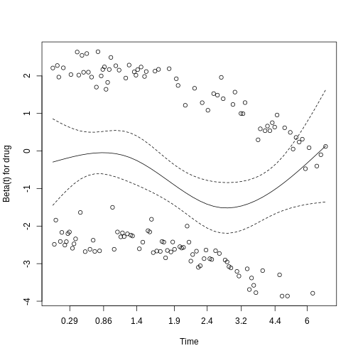
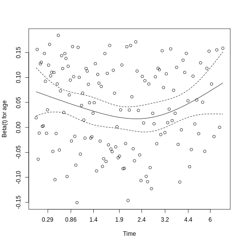
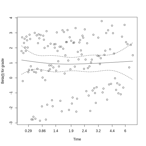
Interpretation:
The output shows a test statistic and p‐value for each covariate and a GLOBAL test.
For each row, p‐value \(<0.05\) indicates that covariate’s hazard ratio varies over time.
A GLOBAL p‐value \(<0.05\) indicates some covariate violates proportional hazards.
Graphs of residuals vs. time (plot(zph_test)) should show a roughly horizontal line under \(H_0\). Trends suggest time‐varying effects.
If all p‐values \(\ge 0.05\), we fail to reject \(H_0\) and conclude the proportional hazards assumption is reasonable.
Aftale- og concordance-mål
EJ KORREKTURLÆST MON IKKE DENNE SNARERE SKAL KONSOLIDERES MED DEN COHENS VI ALLEREDE HAR?
-
Used for Quantifying agreement between two raters
classifying the same subjects into categories, beyond chance.
- Real-world example: Assessing whether two pathologists agree on “Benign” vs. “Malignant” diagnoses.
Assumptions * Each subject is independently rated by
both raters.
* Ratings are categorical (nominal or ordinal).
* The marginal distributions of categories need not be equal.
Strengths * Corrects for agreement expected by
chance.
* Provides an interpretable coefficient, \(\kappa\), ranging from –1 to 1.
* Can be weighted for ordinal categories.
Weaknesses * Sensitive to prevalence and marginal
imbalances (“paradox”).
* Doesn’t distinguish systematic bias from random disagreement.
* Requires at least two raters and non‐sparse tables for stable
estimates.
Example
-
Null hypothesis (\(H_{0}\)): \(\kappa = 0\) (no agreement beyond
chance).
- Alternative hypothesis (\(H_{1}\)): \(\kappa \neq 0\) (agreement beyond chance).
R
# install.packages("psych")  # if necessary
library(psych)
OUTPUT
Attaching package: 'psych'OUTPUT
The following objects are masked from 'package:DescTools':

    AUC, ICC, SD
OUTPUT
The following objects are masked from 'package:ggplot2':

    %+%, alpha
OUTPUT
The following object is masked from 'package:car':

    logit
R
set.seed(2025)
n <- 50
# Simulate two raters classifying subjects as "Yes" or "No":
rater1 <- sample(c("Yes","No"), n, replace = TRUE, prob = c(0.6,0.4))
# Rater2 agrees 70% of the time:
rater2 <- ifelse(runif(n) < 0.7,
                 rater1,
                 ifelse(rater1=="Yes","No","Yes"))

ratings    <- data.frame(rater1, rater2)
kappa_result <- cohen.kappa(ratings)

# Display results:
kappa_result
OUTPUT
Call: cohen.kappa1(x = x, w = w, n.obs = n.obs, alpha = alpha, levels = levels,
    w.exp = w.exp)

Cohen Kappa and Weighted Kappa correlation coefficients and confidence boundaries
                 lower estimate upper
unweighted kappa 0.077     0.34   0.6
weighted kappa   0.077     0.34   0.6

 Number of subjects = 50
Interpretation The estimated Cohen’s \(\kappa\) is
\(\widehat{\kappa}\) = 0.3377
The test statistic (z) = kappa_result$z[1] DETTE FUNGERER IKKE - Z ER IKKE I OBJEKTET.
with p-value =\(\texttt{signif(kappa_result\$p.value[1], 3)}\). DET HER FUNGERER VIST HELLER IKKE…
Since p = r signif(kappa_result$p.value[1], 3) EJ HELLER DETTE
If p < 0.05, we reject \(H_{0}\) and conclude there is agreement beyond chance.
If p ≥ 0.05, we fail to reject \(H_{0}\) and conclude no evidence of agreement beyond chance.
Conventionally, \(\kappa\) values are interpreted as:
0.01–0.20: slight agreement
0.21–0.40: fair agreement
0.41–0.60: moderate agreement
0.61–0.80: substantial agreement
0.81–1.00: almost perfect agreement
EJ KORREKTURLÆST
-
Used for Assessing the reliability or agreement of
quantitative measurements made by two or more raters.
- Real-world example: Determining how consistently three radiologists measure tumor size on MRI scans.
Assumptions:
- Measurements are continuous and approximately normally
distributed.
- Raters are randomly selected (for the “random‐effects” model) or fixed (for the “fixed‐effects” model), depending on choice.
- No interaction between subjects and raters (i.e., rater effects are consistent across subjects).
- Balanced design: each subject is rated by the same set of raters.
Strengths
- Quantifies both consistency and absolute agreement, with different
model/type options.
- Can accommodate any number of raters and subjects.
- Provides confidence intervals and tests for ICC.
Weaknesses
- Sensitive to violations of normality and homogeneity of
variance.
- Choice of model (one‐way vs. two‐way) and type (consistency
vs. agreement) affects results.
- Requires balanced data; missing ratings complicate estimation.
Example
-
Null hypothesis (H₀): The intraclass correlation
coefficient ICC = 0 (no reliability beyond chance).
- Alternative hypothesis (H₁): ICC > 0 (measurements are more reliable than chance).
R
library(irr)

# Simulate ratings of 10 subjects by 3 raters:
set.seed(42)
ratings <- data.frame(
  rater1 = round(rnorm(10, mean = 50, sd = 5)),
  rater2 = round(rnorm(10, mean = 50, sd = 5)),
  rater3 = round(rnorm(10, mean = 50, sd = 5))
)

# Compute two-way random effects, absolute agreement, single rater ICC:
icc_result <- icc(ratings,
                  model = "twoway",
                  type  = "agreement",
                  unit  = "single")

# Display results:
icc_result
OUTPUT
 Single Score Intraclass Correlation

   Model: twoway
   Type : agreement

   Subjects = 10
     Raters = 3
   ICC(A,1) = -0.0823

 F-Test, H0: r0 = 0 ; H1: r0 > 0
  F(9,16.8) = 0.77 , p = 0.645

 95%-Confidence Interval for ICC Population Values:
  -0.326 < ICC < 0.382
Interpretation:
The estimated ICC is -0.08 with a 95% CI [-0.33, 0.38] and p-value = 0.645. We fail to reject the null hypothesis. This indicates that there is no evidence of reliability beyond chance among the raters.
EJ KORREKTURLÆST
- Used for Assessing agreement between two quantitative measurement methods by examining the mean difference (bias) and the limits of agreement. It tests if any difference is constant across the range of measurements, and if there is heteroskedasticity in the data (are there differences that are dependent on measurement levels)
- Real-world example: Comparing blood pressure readings from a new wrist monitor and a standard sphygmomanometer.
Assumptions * Paired measurements on the same
subjects.
* Differences (method A – method B) are approximately normally
distributed.
* No strong relationship between the magnitude of the measurement and
the difference (homoscedasticity).
Strengths * Provides both a visual (Bland–Altman
plot) and numerical summary (bias and limits) of agreement.
* Easy to interpret clinically: shows how far apart two methods can
differ for most observations.
* Does not rely on correlation, which can be misleading for
agreement.
Weaknesses * Assumes constant bias across range of
measurements.
* Sensitive to outliers, which can widen limits of agreement.
* Requires adequate sample size (n ≥ 30 preferred) to estimate limits
reliably.
Example
-
Null hypothesis (H₀): Mean difference between
methods A and B is zero (no systematic bias).
- Alternative hypothesis (H₁): Mean difference ≠ 0 (systematic bias exists).
R
# Simulated paired blood pressure measurements (mmHg) on 12 subjects:
wrist   <- c(120, 122, 118, 121, 119, 117, 123, 120, 118, 119, 122, 121)
sphyg   <- c(119, 121, 117, 122, 118, 116, 124, 119, 117, 120, 121, 122)

# Compute differences and means:
diffs    <- wrist - sphyg
means    <- (wrist + sphyg) / 2

# Calculate bias and limits of agreement:
bias     <- mean(diffs)
sd_diff  <- sd(diffs)
loa_up   <- bias + 1.96 * sd_diff
loa_low  <- bias - 1.96 * sd_diff

# Test for zero bias:
t_test   <- t.test(diffs, mu = 0)

# Bland–Altman plot:
library(ggplot2)
ba_df <- data.frame(mean = means, diff = diffs)
ggplot(ba_df, aes(x = mean, y = diff)) +
  geom_point() +
  geom_hline(yintercept = bias,    linetype = "solid") +
  geom_hline(yintercept = loa_up,   linetype = "dashed") +
  geom_hline(yintercept = loa_low,  linetype = "dashed") +
  labs(title = "Bland–Altman Plot",
       x = "Mean of Wrist & Sphyg Measurements",
       y = "Difference (Wrist – Sphyg)")
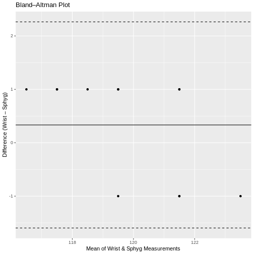
R
# Print numerical results:
bias; loa_low; loa_up; t_test
OUTPUT
[1] 0.3333OUTPUT
[1] -1.597OUTPUT
[1] 2.263OUTPUT
	One Sample t-test

data:  diffs
t = 1.2, df = 11, p-value = 0.3
alternative hypothesis: true mean is not equal to 0
95 percent confidence interval:
 -0.2923  0.9590
sample estimates:
mean of x
   0.3333
Interpretation The mean difference (bias) is 0.33 units, with 95% limits of agreement from -1.6 to 2.26 units. The t-test for zero bias yields a p-value of 0.266, so we fail to reject the null hypothesis. This indicates that there is no statistically significant bias; the two methods agree on average.
Der skal nok suppleres med: Weighted κ is used for ordinal values. We use the function kappa2() from the irr package. Light’s κ is used for studying interrater agreement between more than 2 raters. We use the function kappamlight() from the irr package. Fleiss κ is also used when having more than 2 raters. But does not require the same raters for each subject.
Little’s test for MCAR. Fra biblioteket naniar
- Use an appropriate statistical test
- Make sure you understand the assumptions underlying the test