Logistic regression
Last updated on 2026-06-15 | Edit this page
Overview
Questions
- How do you run a logistic regression?
- What is the connection between odds and probabilities?
Objectives
- Learn how to run a logistic regression
OUTPUT
── Attaching core tidyverse packages ──────────────────────── tidyverse 2.0.0 ──
✔ dplyr     1.2.1     ✔ readr     2.2.0
✔ forcats   1.0.1     ✔ stringr   1.6.0
✔ ggplot2   4.0.3     ✔ tibble    3.3.1
✔ lubridate 1.9.5     ✔ tidyr     1.3.2
✔ purrr     1.2.2
── Conflicts ────────────────────────────────────────── tidyverse_conflicts() ──
✖ dplyr::filter() masks stats::filter()
✖ dplyr::lag()    masks stats::lag()
ℹ Use the conflicted package (<http://conflicted.r-lib.org/>) to force all conflicts to become errors
Logistic Regression
Using linear regression, or even non-linear multiple regression techniques, we can predict the expected value of a dependent continuous variable given values of one or more independent variables.
But what if the dependent variable we want to predict is not continous, but categorical?
Eg, if we try to predict an outcome like “Healthy/Sick” based on a number of independent variables?
We do that using the logistic regression. Strictly speaking the logistic model does not predict a yes/no answer, but rather the probability that the answer is yes (and conversely that it is no). Rather than the continous outcome the linear methods model for the dependent variable, the logistic regression returns a probability. By definition that lies somewhere between 0 and 1 (or 0% and 100%).
And since the linear methods we would like to use for doing the actual logistic regression does not play nice with those bounds, we need to think about probabilities in a different way.
A new way of thinking about probability.
We often talk about there being a “67%” probability or chance of something. Reading p-values, we do that all the time. A p-value of 0.05, equivalent to 5%, tells us that if we run the test often enough, there is a 5% chance of seeing a result as extreme as the test value purely by chance, if the null-hypothesis is true.
5% is equivalent to 5 instances out of 100 possibilities. As indicated above, we want to convert those 5% to something that does not have a range between 0 and 1.
Therefore, we convert probabilities to odds.
Odds are a different way of representing probabilities. A lot of statistics and probability theory have their roots in gaming and betting, so let us use that as an example.
If two soccer-teams play, and we want to bet on the outcome, the betting company we place our bet at, will give us odds. 1:9 indicates that if the two teams play 10 times, one team will win 1 game, and the other will win 9 times (assuming that a tie is not possible, and glossing over a lot of other details that relates more to the companys profits). That is equivalent to one team having a 10% chance of winning, and the other having a 90% chance of winning.
The connection between the two numbers is found by:
\[odds = \frac{p}{1-p}\]
We have now transformed a probability going between 0 and 1, to odds, that can go between 0 and positive infinity.
Going a step further
Modelling probabilities is difficult, because they can only have values between 0 and 1. Converting them to odds, give us something that can have values between 0 and infinity (positive). If we take one extra step, we can convert those odds to something that is continuous and, can have any value.
We do that by taking the (natural) logarithm of the odds, and the entire conversion from probability to log-odds, is called the logit-function:
\[logit(p) = \log(\frac{p}{1-p})\]
Challenge
Remember the probabilities of the soccer-match? One team had a 10% probability of winning, corresponding to odds 1:9. That means that the other team have a 90% probability of winning, or odds 9:1. Try to run the logit function on both of those probabilities. Do you notice a nice relation between them?
R
log(0.1/(1-0.1))
OUTPUT
[1] -2.197225R
log(0.9/(1-0.9))
OUTPUT
[1] 2.197225The two log-odds values have different signs, but are otherwise identical. This is nice and symmetrical.
So - what are we modelling?
This:
\[\text{logit}(p) = \beta_0 + \beta_1 X_1 + \beta_2 X_2 + \dots + \beta_k X_k\]
And that looks familiar, and the net result of all the stuff about odds, logit-functions etc. have exactly that as their goal; we can now use all the nice techniques from the linear regressions to model categorical values.
It’s not exactly that simple. In the linear regression we fit the data to a line, where we in the logistic regression fits the data to a sigmoid curve:
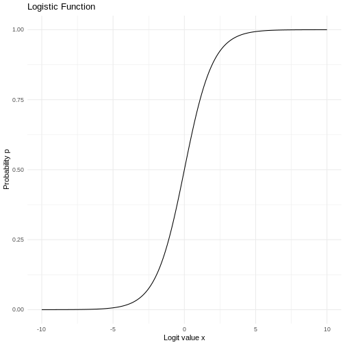
OK, lets make a fit already!
We start be getting some data. Download the FEV dataset, but start by creating a folder called “data”:
R
download.file("https://raw.githubusercontent.com/KUBDatalab/R-toolbox/main/episodes/data/FEV.csv", "data/FEV.csv", mode = "wb")
OUTPUT
Rows: 654 Columns: 6
── Column specification ────────────────────────────────────────────────────────
Delimiter: ","
dbl (6): Id, Age, FEV, Hgt, Sex, Smoke

ℹ Use `spec()` to retrieve the full column specification for this data.
ℹ Specify the column types or set `show_col_types = FALSE` to quiet this message.
R
fev <- read_csv("data/FEV.csv")
The data contains measurements of age, height, sex and lung function for 654 children, as well as an indication of wether or not they smoke.
R
fev
OUTPUT
# A tibble: 654 × 6
      Id   Age   FEV   Hgt   Sex Smoke
   <dbl> <dbl> <dbl> <dbl> <dbl> <dbl>
 1   301     9  1.71  57       0     0
 2   451     8  1.72  67.5     0     0
 3   501     7  1.72  54.5     0     0
 4   642     9  1.56  53       1     0
 5   901     9  1.90  57       1     0
 6  1701     8  2.34  61       0     0
 7  1752     6  1.92  58       0     0
 8  1753     6  1.42  56       0     0
 9  1901     8  1.99  58.5     0     0
10  1951     9  1.94  60       0     0
# ℹ 644 more rows
We will do a logistic regression, to see if we can predict wether or not a child is smoking, based on all the other variables (except the Id value).
As both Sex and Smoke are categorical values, it is important that they are actually coded as categorical values in the data, in order for R to be able to handle them as such:
R
fev <- fev |>
  mutate(Sex = factor(Sex),
         Smoke = factor(Smoke))
We can now build a model. It looks almost like the linear model, but
rather than using the lm() function we use the
glm(), or “generalised linear model”, which is able to
handle logistic models. It is general, so we need to specify
that we are running a binomial (ie two possible outcomes) fit. We save
the result to an object, so we can take a closer look:
R
log_model <- glm(Smoke ~ Age + FEV + Hgt + Sex, family = "binomial", data = fev)
The result in itself looks like this:
R
log_model
OUTPUT
Call:  glm(formula = Smoke ~ Age + FEV + Hgt + Sex, family = "binomial",
    data = fev)

Coefficients:
(Intercept)          Age          FEV          Hgt         Sex1
   -18.6141       0.4308      -0.5452       0.2122      -1.1652

Degrees of Freedom: 653 Total (i.e. Null);  649 Residual
Null Deviance:	    423.4
Residual Deviance: 300 	AIC: 310
And if we take a closer look:
R
summary(log_model)
OUTPUT
Call:
glm(formula = Smoke ~ Age + FEV + Hgt + Sex, family = "binomial",
    data = fev)

Coefficients:
             Estimate Std. Error z value Pr(>|z|)
(Intercept) -18.61406    3.51282  -5.299 1.17e-07 ***
Age           0.43075    0.07098   6.069 1.29e-09 ***
FEV          -0.54516    0.31662  -1.722 0.085103 .
Hgt           0.21224    0.06371   3.331 0.000865 ***
Sex1         -1.16517    0.38943  -2.992 0.002772 **
---
Signif. codes:  0 '***' 0.001 '**' 0.01 '*' 0.05 '.' 0.1 ' ' 1

(Dispersion parameter for binomial family taken to be 1)

    Null deviance: 423.45  on 653  degrees of freedom
Residual deviance: 300.02  on 649  degrees of freedom
AIC: 310.02

Number of Fisher Scoring iterations: 7
Interestingly lungfunction does not actually predict smoking status very well.
But what does the coefficients actually mean?
The intercept is not very interesting in itself, and we do not generally interpret directly on it. It represents the log-odds of smoking if all the predictive variables (Age, FEV, Hgt, and Sex) are 0. And the log-odds in that case is not very informative.
We have a positive coefficient for Age. That means, that for each unit increase in age, here 1 year, the log-odds for smoking increase by 0.43075, if all other variables are kept constant. Since we have log-odds, we can find the increase in odds for smoking by taking the exponential of the log-odds:
R
exp(0.43075)
OUTPUT
[1] 1.538411That is - the odds for smoking increase by 53.8% for each year a child get older.
The coefficients for FEV and Hgt are treated similarly. Note that for FEV, the coefficient is negative. That means the log-odds, and therefore odds, for smoking decreases as lungfunction measured by FEV, increases. As always if all other variables are kept constant.
Sex is a bit different. Because Sex is a categorical variable, the coefficient indicates that there is a difference between the two different sexes. And because it is negative, we can calculate that the odds for smoking if the child is female is
R
exp(-1.16517)
OUTPUT
[1] 0.3118696compared with male childre, equivalent to a reduction in odds by about 68.8%
How to get the odds quickly?
We can get the odds in one go, rather than running the exponential function on them one by one:
R
exp(coef(log_model))
OUTPUT
 (Intercept)          Age          FEV          Hgt         Sex1
8.241685e-09 1.538413e+00 5.797479e-01 1.236439e+00 3.118701e-01
We use the coef() function to extract the coefficients,
and then take the exponential on all of them.
And what about the probabilities?
Sometimes it would be nice to get probabilities instead of odds. We can get those using this expression:
R
1/(1+exp(-coef(log_model)))
OUTPUT
 (Intercept)          Age          FEV          Hgt         Sex1
8.241685e-09 6.060530e-01 3.669876e-01 5.528606e-01 2.377294e-01
And interpreting the probabilities?
A probability of 0.606 means that for each unit increase in Age, the probabililty of the the outcome “smoking” increases by 60.6%
A probablity of 0.367 means that for each unit increase in FEV, the probability of that outcome decreases by 36.7%
What about the p-values?
p-values in logistic regression models are interpreted in the same way as p-values in other statistical tests:
Given the NULL-hypothesis that the true value for the coefficient for FEV in our model predicting the odds for smoking/non-smoking, is 0.
What is the probability of getting a value for the coefficient that is as extreme as -0.54516?
If we run the experiment, or take the sample, often enough, we will see a coefficient this large, or larger (in absolute values), 8.5% of the times. If we decide that the criterium for significanse is 5%, this coefficient is not significant.
Predictions
We generally experience that students are not really interested in predicting an outcome. However part of the rationale behind building these models is to be able to predict - outcomes.
Given a certain age, height, FEV and sex of a child, what is the log-odds of that child smoking?
The easiest and most general way of predicting outcomes based on a
model, is to use the predict() function in R.
It takes a model, and some new data, and returns a result.
We begin by building a dataframe containing the new data:
R
new_child <- data.frame(Age = 13, Hgt = 55, FEV = 1.8, Sex = factor(1, levels = c(0,1)))
Here we are predicting on a boy (Sex = 1), aged 13, with a lungvolume of 1.8l and a height of 55 inches.
It is important that we use the same units as the model. That is, we need to use inches for the height, liters for the lung volume, and the correct categorical value for Sex.
Now we plug that into the predict function, along with the model:
R
predict(log_model, newdata = new_child)
OUTPUT
        1
-3.487813
This will return the predicted log-odds, and we can either calculate the probability from that. Or we can add a parameter to the predict model, to the the probability directly:_
R
predict(log_model, newdata = new_child, type = "response")
OUTPUT
         1
0.02966099 Do the conversion yourself
Convert the predicted log-odds to a probability
We run the prediction:
R
predicted_odds <- predict(log_model, newdata = new_child)
And then:
R
1/(1+exp(-predicted_odds))
OUTPUT
         1
0.02966099 What about another child?
What is the probability for smoking for a 10 year old 110 cm tall girl, with a lung volume of 1.1 liter?
Begin by making a dataframe describing the girl:
R
new_girl <- data.frame(Age = 10, Hgt = 110/2.54, FEV = 1.1, Sex = factor(0, levels = c(0,1)))
And use predict() with the correct type
argument to get the result directly:
R
predict(log_model, newdata = new_girl, type = "response")
OUTPUT
          1
0.003285539 - Using the predict-function to predict results is the easier way