Histograms

Last updated on 2025-07-01 | Edit this page

Overview

Questions

What is a histogram?
What do we use histograms for?
What is the connection between number of bins, binwidths and breaks?
How do we chose a suitable number of bins?

Objectives

Understand what a histogram is, and what it is used for
Introduce a number of heuristics for chosing the “correct” number of bins

What even is a histogram?

We use histograms to visualise the distribution of some continuous variable. It have values between a minimum and maximum value (range), but are these values equally probable? Probably not.

In a histogram we divide the range in a number of bins, count the number of observations in each bin, and make a plot with a bar for each bin, where the height is equivalent to the number of observations in each bin.

Normally the bins have equal width - equal to the range of the variable (max - min), divided by the number of bins.

How do we do that?

Let us look at some data - penguin data:

R

library(tidyverse)
library(palmerpenguins)

R has a build-in histogram function, hist(), which will make a basic histogram, of the data we provide it with:

R

hist(penguins$bill_length_mm)

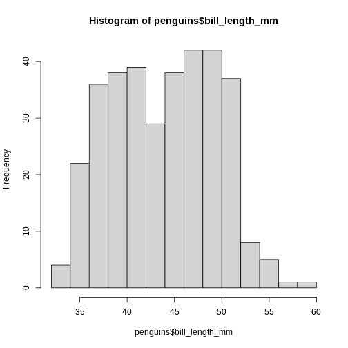
This is not a very nice looking histogram, and ggplot2 provides us with a more easily customisable geom_histogram() function:

R

ggplot(penguins, aes(x=bill_length_mm)) +
  geom_histogram()

OUTPUT

`stat_bin()` using `bins = 30`. Pick better value with `binwidth`.

WARNING

Warning: Removed 2 rows containing non-finite outside the scale range
(`stat_bin()`).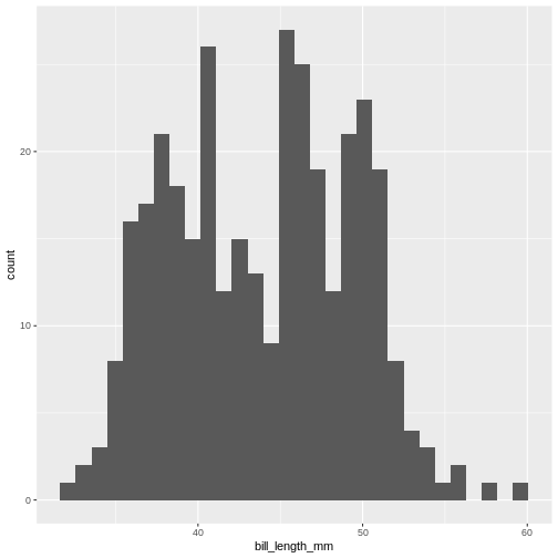

This is the distibution of the length, in millimeter, of the bill (or beak) of a selection of penguins.

By default the geom_histogram() function divides the range of the data (min = 32.1, max = 59.6 mm) into 30 bins. Each bin therefore have a width of 0.9167 mm. The first bin contains a single penguin, that has a beak that is between 32.1 and 32.1 + 0.9187 mm long.

From this plot we get information about the distribution of bill-lengths of penguins.

There appears to be several different “peaks” in the plot. This is to be expected as we have three different species of penguins in the data, in addition to having penguins of both sexes.

If we want to split the histogram into these different groups, we can use the possibilities available in ggplot2:

R

ggplot(penguins, aes(x=bill_length_mm)) +
  geom_histogram() +
  facet_grid(sex~species)

OUTPUT

`stat_bin()` using `bins = 30`. Pick better value with `binwidth`.

WARNING

Warning: Removed 2 rows containing non-finite outside the scale range
(`stat_bin()`).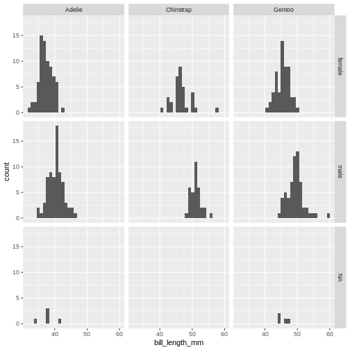

The data now looks a bit more normally distributed. And we can observe that male penguins tend to have longer beaks than female penguins. We can also see that the different species of penguins have different bill lengths.

How many bins?

Note the warning we get.

“using bins = 30. Pick better value with binwidth”

The choice of number of bins have a big influence on how the data is visualised. By providing the geom_histogram() function with an argument, bins = xx where xx is the number of bins we can adjust the number of bins:

Try it yourself

Try to plot the bill_length_mm variable in the penguins dataset with different numbers of bins.

Show me the solution

R

ggplot(penguins, aes(x=bill_length_mm)) +
  geom_histogram(bins = 20)

WARNING

Warning: Removed 2 rows containing non-finite outside the scale range
(`stat_bin()`).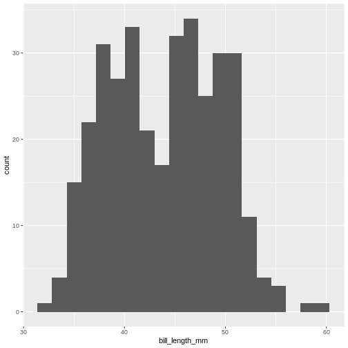

By default geom_histogram() choses 30 bins. This default value has been chosen because it is almost never the correct choice. ggplot2 is an opinionated package, that tries to force us to make better plots. And this is the reason for the warning.

How many bins should we chose?

We should chose the number of bins that best tells the story we want to tell about our data. But also the number of bins that does not hide information about our data.

The obvious way to do this is to fiddle with the number of bins, and find the number that best do that.

But that can feel a bit cheaty. How do we rationalise the number of bins in a way that makes sure that this number is not just the one that show what we want the data to show, but the number that actually show the data as it is?

A number of heuristics for chosing the “correct” number of bins exist.

Why do we call it a heuristic?

A heuristic is a fancy way of saying “rule of thumb”. “Heuristic” sounds like we know what we are talking about.

Different heuristics for chosing number of bins.

To have an approximately consistent way of describing them, we use these three values:

k for the number of bins
h for the width of the bins
n for the number of observations

We also use a couple of mathematical signs: \(\lceil\) and \(\rceil\). These are “ceiling” functions, and simply mean that we round a number up. Rather than rounding 4.01 to 4, we round up to 5.

Freedman-Diaconis

This heuristic determines the bind-width as:

\[h = 2 \cdot IQR \cdot n^{-1/3}\] where IQR is the interquartile range of our data, which can be found using the IQR() function.

The number of bins are then found as

\[ k = \lceil \frac{range}{h} \rceil \] ::::challenge ## Try it yourself

How many bins does Freedman-Diaconis prescribe for making a histogram of the bill length of the penguins?

Show me the solution

Get all the lengths of the penguin bills, excluding missing values:

R

bill_lengths <- penguins$bill_length_mm %>% 
  na.omit()

Find \(n\):

R

n <- length(bill_lengths)

And the inter quartile range:

R

iqr <- IQR(bill_lengths)

Now find the recommended bin-width:

R

h <- 2*iqr*n^(-1/3)

And then the number of bins:

R

k <- (max(bill_lengths) - min(bill_lengths))/h

Remember to take the ceiling:

R

ceiling(k)

OUTPUT

[1] 11

::::

Square root rule

The number of bins \(k\) are found directly from the number of observations, n:

\[k = \lceil\sqrt{n}\rceil\]

Try it yourself

According to the Square Root rule, how many bins should we use for a histogram of the length of penguin bills?

Show me the solution

Get all the lengths of the penguin bills, excluding missing values:

R

bill_lengths <- penguins$bill_length_mm %>% 
  na.omit()

Find \(n\):

R

n <- length(bill_lengths)

And calculate the square root of \(n\), rounded up using the ceiling() function:

R

ceiling(sqrt(n))

OUTPUT

[1] 19

The Sturges rule

Here we also find \(k\) directly from the number of observations:

\[ k = \lceil\log_2(n) + 1\rceil \] An implicit assumption is that the data is approximately normally distributed.

\(\log_2\) is found using the log2() function.

Try it yourself

According to the Sturgess rule, how many bins should we use for a histogram of the length of penguin bills?

Show me the solution

Get all the lengths of the penguin bills, excluding missing values:

R

bill_lengths <- penguins$bill_length_mm %>% 
  na.omit()

Find \(n\):

R

n <- length(bill_lengths)

Now find \(k\)

R

k <- log2(n) + 1

And remember to round up:

R

ceiling(k)

OUTPUT

[1] 10

The Rice Rule

Again we get \(k\) directly from \(n\):

\[k = \lceil 2n^{1/3}\rceil\] ::::challenge

According to the Rice rule, how many bins should we use for a histogram of the length of penguin bills? ::::solution

Get all the lengths of the penguin bills, excluding missing values:

R

bill_lengths <- penguins$bill_length_mm %>% 
  na.omit()

Find \(n\):

R

n <- length(bill_lengths)

And then find \(k\):

R

k <- 2*n^(1/3)

Remember to round up:

R

ceiling(k)

OUTPUT

[1] 14

:::: ::::

Doanes Rule

This rule is a bit more complicated:

\[k= 1 + \log_2(n) + \log_2(1+ |g_1|/\sigma_{g1})\]

\(|g_1|\) is the absolute value of the estimated 3rd moment skewness of the data, found by using the skewness() function from the e1071 package, and \(\sigma_{g1}\) is found by:

\[\sigma_{g1} = \sqrt{6(n-2)/((n+1)(n+3))}\]

Doanes rule basically adds extra bins based on how skewed the data is, and works better than Sturges’ rule for non-normal distributions.

Challenge

According to Doanes rule, how many bins should we use for a histogram of the length of penguin bills? ::::solution

Get all the lengths of the penguin bills, excluding missing values:

R

bill_lengths <- penguins$bill_length_mm %>% 
  na.omit()

Find \(n\):

R

n <- length(bill_lengths)

Find \(g_1\):

R

g1 <- skewness(bill_lengths)

ERROR

Error in skewness(bill_lengths): could not find function "skewness"

Find \(\sigma_{g1}\):

R

s_g1 <- sqrt(6*(n-2)/((n+1)*(n+3)))

Now we can find \(k\). Remember to take the absolute value of \(g_1\)

R

k <- 1 + log2(n) + log2(1+abs(g1)/s_g1)

ERROR

Error: object 'g1' not found

And then round up \(k\) to get the number of bins:

R

ceiling(k)

OUTPUT

[1] 14

::::

Scott’s rule

Here we get the bin-width \(h\) using this expression:

\[h = 3.49 \frac{\sigma}{n^{1/3}}\] Where \(\sigma\) is the standard deviation of the data. This rule implicitly assumes that the data is normally distributed.

Challenge

According to Scott’s rule, how many bins should we use for a histogram of the length of penguin bills? ::::solution

Get all the lengths of the penguin bills, excluding missing values:

R

bill_lengths <- penguins$bill_length_mm %>% 
  na.omit()

Find \(n\):

R

n <- length(bill_lengths)

Find \(\sigma\):

R

sigma <- sd(bill_lengths)

Now we can find the bin-width \(h\):

R

h <- 3.49*sigma*(n^(-1/3))

And from that, the number of bins \(k\):

R

k <- (max(bill_lengths) - min(bill_lengths))/h

Remember to round up \(k\):

R

ceiling(k)

OUTPUT

[1] 11

::::

That is difficult

Rather than doing these calculations on our own, we can read the help file for the hist() function. The argument breaks allow us to specify where the breaks in the histogram - the splits in bins - should occur.

We can see that the default value is “Sturges”. And under details we can see the other options that hist() can work with, “Scott” and “FD” for Freedman-Diaconis. We also get a hint of the functions that can return the number of bins:

R

nclass.Sturges(penguins$bill_length_mm)

OUTPUT

[1] 10

nclass.FD and nclass.scott works similarly, but note that it is necessary to remove missing values. If one of the other heuristics is needed, we either need to do the calculations ourself - or try to identify a package that contains functions to do it.

Another way

With these heuristics, we can calculate the recommended number of bins for making a histogram. And with that number, knowing the range of the data, we can calculate the binwidth.

Either of those can be used as an argument in geom_histogram(), bins= and binwidth= respectively.

However, for effective communication, we might consider a third way. The bill length of the penguins ranges from 32.1 to 59.6 mm. With 9 bins we will get a bin width of 3.055556 mm. The first bin will therefore start at 32.1 and end at 35.15556 mm, and the second will start at 35.15556 mm and end at 38.21112. These are the breaks, and they are not very intuitive.

Instead we might consider choosing the breaks ourself. Having a first bin that starts at 32 mm and ends at 35, and the a second bin that starts at 35 mm and ends at 38 might be beneficial for understanding the histogram.

Those breaks can also be provide to the geom_histogram() function - we just need to calculate them our self.

The seq() function is useful for this.

This function returns a sequence of numbers from a start value, to and end value, in steps that we can chose:

R

seq(from = 30, to = 65, by = 5)

OUTPUT

[1] 30 35 40 45 50 55 60 65

You will have to think about the from and the to arguments, to not exclude any observations, but this method give us much more natural breaks in the histogram:

R

penguins %>% 
  ggplot(aes(x=bill_length_mm)) +
  geom_histogram(breaks = seq(from = 30, to = 65, by = 5))

WARNING

Warning: Removed 2 rows containing non-finite outside the scale range
(`stat_bin()`).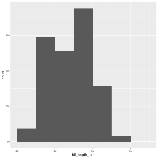

Do not abuse the option of specifying breaks!

Instead of using the seq() function we could construct the breaks by hand:

R

c(30, 35, 40, 45, 50, 55, 60, 65)

And it might be tempting enter breaks that would lead to uneven binwidths:

R

c(30, 40, 42, 45, 50, 55, 60, 65)

Do not do this. This will, except in very rare cases, rightfully be considered misleading. Always use a consistent binwidth!

Key Points

Histograms are used for visualising the distribution of data
A lot of different rules for chosing number of bins exists
Binwidth and number of bins are equivalent
Chose the number of bins that best supports your data story. Without hiding inconvenient truths about your data.
Never use unequal binwidths
Consider using natural breaks as an alternative