A deeper dive into pipes

Last updated on 2025-07-01 | Edit this page

Overview

Questions

What are the differences between the two pipes?

Objectives

Explain some of the differences between the two families of pipes

Almost everywhere in this course material, you will see the pipe.

But the story about the pipe is larger than %>%.

The %>% version come from the magrittr package, and was introduced to the R-world in 2014. It became one of the defining features of the R-dialect “tidyverse”. It proved useful enough that a similar pipe |> was introduced in “base-R” with version 4.1 in May 2021.

R dialects

R-programmers tend to write in one dialect of R, small variations that are understandable - but still different. The three common dialects are “base R”, the tidyverse and data.table. One of the defining features of the tidyverse dialect has been the magrittr pipe. This differences is eroding with the introduction of the native pipe in base R.

KUB Datalab speaks the tidyverse dialect, and will continue to use the magrittr pipe until the default keyboard shortcut to the pipe in RStudio changes

The base-R pipe function in a similar way to the magrittr pipe. But there are differences:

Topic	Magrittr 2.0.3	Base 4.3.0	note
Operator	`%\>% %\<\>% %$% %!>% %T>%`	`\|>`	1
Function calls	`1:2 %>% sum()`	`1:2 \|> sum()`
	`1:2 %>% sum`	Needs the parentheses
	`1:3 %>%``+` `4`	Not every function is supported
Insert on first empty place	`mtcars %>% lm(formula=mpg ~ disp)`	`mtcars \|> lm(formula = mpg ~ disp)`	2
placeholder	.	_
	`mtcars %>% lm(mpg~disp, data = .)`	`mtcars \|> lm(mpg ~ disp, data = _)`
	`mtcars %>% lm(mpg~disp, .)`	Needs named argument	3
	`1:3 %>% setNames(., .)`	Can only appear once
	`1:3 %>% {sum(sqrt(.))}`	Nested calls not allowed	4
Extraction call	`mtcars %>% .$cyl` `mtcars %>% {.$cyl[[3]]}` `mtcars %$% cyl[[3]]`	`mtcars \|> _$cyl` `mtcars \|> _$cyl[[3]]`
Environment	`%>%` has additional function environment. Use: `"x" %!> assign(1)`	`"x" \|> assign(1)`	4
Create Function	`top6 <- . %>% sort() %>% tail()`	Not possible
Speed	Slower because overhead of function call	Faster because syntax transformation	5

Unless we explicitly import the magrittr package, we typically only have access to the simple pipe, %>% which is included in many packages. This however is only one of several pipes available from the magrittr package. See below.
Note that both pipes insert the input from the left-hand-side at the first unnamed argument. Naming other arguments allow us to handle functions that do not take data as the first argument.
The placeholder allow us to reference the input in functions. One important difference is that the base-R pipe need to be specified with a named argument. Which is probably best practice anyway.
This is related to the way the pipes actually work, see also 5.
The magrittr pipe works by rewriting the right-hand-side in a function, with its own environment - where the left-hand-side is available with the symbol `.`

The other pipes

As indicated in the comparative table, the magrittr pipe have a number of siblings.

The tee-pipe %T>%

This pipe allow us to inject a function into a longer set of pipes, without affecting the rest of the flow.

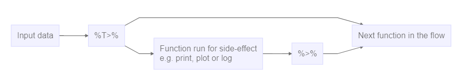
The tee-pipe sends data to two functions. The immediate next, which we want to run for plotting, logging or printing data, and to the next function over, which get the original input data, rather than what is returned by the intermediate function.

We are here using an intermediate function, not for what it does to the data, but for its side effects.

Try it yourself

Use the tee-pipe to send the dataset mtcars to a view function, and then filter to only show rows where am is equal to 1.

Show me the solution

R

mtcars %T>%
  view() %>% 
  filter(am == !)

Assignment pipen

After constructing a longer pipe in order to get at specific result, we end up assigning the result to a new object. Sometimes the same object:

R

my_data <- my_data %>% 
  filter(lending > 10) %>% 
  mutate(area = lenght * width)

The assignment pipe can shorten this:

R

my_data %<>% 
  filter(lending > 10) %>% 
  mutate(area = lenght * width)

It needs to be the first pipe in the flow, and will pass the data from its left hand side to the flow on the right hand side. And assign the result of the entire pipe back into the original left hand side.

This will shorten your code. But it is generally recommended not to use it.

Reading R-code can be difficult enough as it is, and %>% is visually rather close to %<>% which makes it easy to overlook.

The eager pipe %!>%

We definitely need an episode in this material that cover the concept of lazy evaluation. But currently we are too lazy to write it.

But. The usual pipe %>% i “lazy”. An expression in a set of pipes is only evaluated when R absolutely have to. This can do weird things, especially if we run functions for their side effects, e.g. when we use the tee-pipe to do logging of intermediate results.

Enter the eager pipe, %!>%. This will force the evaluation rather than postpone it to later.

Let us define three functions. The code is not that important, but they take an input, prints a text indicating their name (ie function f prints “function f”), and return the input unchanged. This printing is the side effect.

Take a look below if you are curious:

Defining three functions

R

f <- function(x) {
  print("function f")
  x
}

g <- function(x) {
  print("function g")
  x
}

h <- function(x) {
  print("function h")
  invisible(x)
}

invisible() returns x, but withou printing it.

We can now run these three functions in a pipe:

R

library(magrittr)

NULL %>% f() %>% g() %>% h()

OUTPUT

[1] "function h"
[1] "function g"
[1] "function f"

This is the lazy evaluation. The first print come from the last function, and function g is only evaluated when it has to be. Because function h needs it. The last function to be evaluated is function f - the first we actually have in the pipes. Because it is only evaluated when needed. That is, when function g needs it.

Eager evaluation, where the functions are not evaluated when needed, but immediately, can be achieved using the eager pipe:

R

NULL %!>% f() %!>% g() %!>% h()

OUTPUT

[1] "function f"
[1] "function g"
[1] "function h"

Now the first message printed is from function f. Becaus function f is the first, and we are using the eager pipe rather than the lazy.

R use lazy evaluation for a reason

It might be tempting to use the eager pipe every time. After all, it is bad to be lazy and the evaluation have to be done at one point, right. But! R, and especially the tidyverse functions use lazy evaluation because it improves performance. If something in the pipe is not actually used, it is not evaluated. This saves time.

The exposition pipe

The power of the pipes comes from the fact that we can use them to forward data to a function that use a dataframe.

But not all functions have an argument that allow them to take a dataframe as input. And because the pipe inserts whatever is on the lefthand side of it, into the first empty argument in the function on the right hand side, this can lead to problems.

Try it yourself

You will fail!

Use the cor() function in conjunction with the ordinary pipe (%>%), to find the correlation between the Sepal.Length and the Sepal.Width in the iris dataset.

Give me a hint

Something like this:

R

iris %>% 
  cor(x = .$Sepal.Length, y = .$Sepal.Width)

Might be tempting. Try to add other named arguments to the function (look at the help file) if you do not succeed at first.

Show me the solution

This cannot be done.

In this attempt:

R

iris %>% 
  cor(x = .$Sepal.Length, y = .$Sepal.Width,
      use = "everything")

We add more and more named arguments to the function. In this code, we will get an error, telling us that we are supplying a dataframe to the argument “method”. Looking at the help, we can see that cor besides the arguments we have already named in the function call, take a final argument “method”. That is the first empty argument in the function, and the pipe will place the dataframe iris on that place, leading to an error. If we supply the method argument inserting method = "pearson", the pipe will still add the dataframe to the function, resulting in an error telling us that we are supplying an argument that is unused.

The exposition pipe, %$% exposes the variables in the left hand side, and does not insert anything anywhere unless we specify it:

R

iris %$% 
  cor(x = Sepal.Length, y = Sepal.Width)

OUTPUT

[1] -0.1175698

That weird note about function calls

In the table comparing the native pipe (|>) and the magrittr pipe (%>%) it was noted that the latter was slower than the first, because of “overhead of function call”. Or conversely that the first was faster because of “syntax transformation”. What does that actually mean?

The magrittr pipe, as are other operators, is a function. Conceptually this a %>% b(), is the same as %>%(a, b())

Or:

R

data %>% 
  filter(x > 0) %>% 
  summarise(mean = mean(y))

become this:

R

`%>%`(`%>%`(data, filter(x > 0)), summarize(mean = mean(y)))

We can count 5 functions, 2 of them the pipe function.

The native pipe on the other hand is not a function. The R-parser, which interprets our code befor actually evaluating it, rewrites code containg the native pipe. That means, that a |> b() becomes b(a)

Or that:

R

data |>
  filter(x > 0) |>
  summarize(mean = mean(y))

become:

R

summarize(filter(data, x > 0), mean = mean(y))

We can count 3 functions in this expression. Intuitively this should be faster. And it is.

What if I want the other pipe?

The keyboard shortcut to get a pipe operator in RStudio is ctrl+shift+m on windows and cmd+shift+m on macos.

This default can be changed:

Tools → Global Options → Code

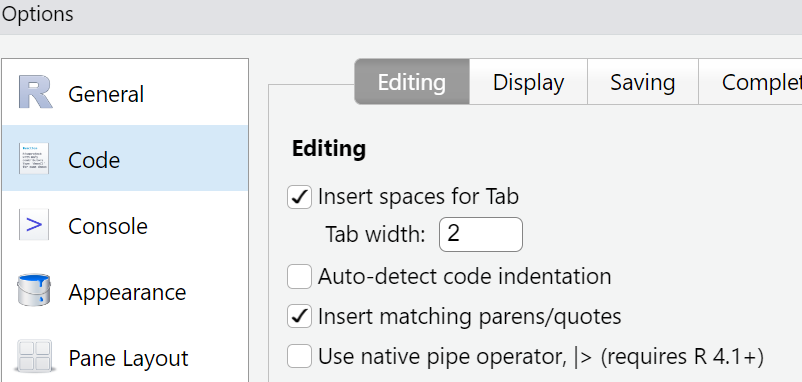Place a tickmark in the box next to “Use native pipe operator, |>”.

Key Points

The base-R, native, pipe |> is faster than the magrittr pipe, %>%
The magrittr package provides a selection of other useful pipes