Factor Analysis
Last updated on 2025-02-04 | Edit this page
Overview
Questions
- How do you write a lesson using R Markdown and sandpaper?
Objectives
- Explain how to use markdown with the new lesson template
- Demonstrate how to include pieces of code, figures, and nested challenge blocks
Minder en del om pca - også i matematikken. Antager at der er et mindre antal underliggende faktorer, som kan forklare observationerne. Det er de underliggende faktorer vi forsøger at belyse. faktoranalysen forklarer kovariansen i data. pca forklarer variansen.
en pca komponent er en lineær kombination af observerede variable. faktoranalysen leder til at de observerede variable er en linear kombination af uobserverede variable eller faktorer.
PCA er dimensionsreducerende. FA finder latente variable.
PCA er en type af faktoranalyse. Men er observationel, mens FA er en modelleringsteknik.
fa kører i to trin. Eksplorativ faktoranalyse, hvor vi identificerer faktorerne. og confirmatory faktoranalyse, hvor vi bekræfter at vi faktisk fik identificeret faktorerne.
Den er vældig brugt i psykologien.
R
library(lavaan)
OUTPUT
This is lavaan 0.6-19
lavaan is FREE software! Please report any bugs.
R
library(tidyverse)
OUTPUT
── Attaching core tidyverse packages ──────────────────────── tidyverse 2.0.0 ──
✔ dplyr     1.1.4     ✔ readr     2.1.5
✔ forcats   1.0.0     ✔ stringr   1.5.1
✔ ggplot2   3.5.1     ✔ tibble    3.2.1
✔ lubridate 1.9.4     ✔ tidyr     1.3.1
✔ purrr     1.0.2
OUTPUT
── Conflicts ────────────────────────────────────────── tidyverse_conflicts() ──
✖ dplyr::filter() masks stats::filter()
✖ dplyr::lag()    masks stats::lag()
ℹ Use the conflicted package (<http://conflicted.r-lib.org/>) to force all conflicts to become errors
R
library(psych)
OUTPUT
Attaching package: 'psych'

The following objects are masked from 'package:ggplot2':

    %+%, alpha

The following object is masked from 'package:lavaan':

    cor2cov
Let us look at some data:
R
glimpse(HolzingerSwineford1939)
OUTPUT
Rows: 301
Columns: 15
$ id     <int> 1, 2, 3, 4, 5, 6, 7, 8, 9, 11, 12, 13, 14, 15, 16, 17, 18, 19, …
$ sex    <int> 1, 2, 2, 1, 2, 2, 1, 2, 2, 2, 1, 1, 2, 2, 1, 2, 2, 1, 2, 2, 1, …
$ ageyr  <int> 13, 13, 13, 13, 12, 14, 12, 12, 13, 12, 12, 12, 12, 12, 12, 12,…
$ agemo  <int> 1, 7, 1, 2, 2, 1, 1, 2, 0, 5, 2, 11, 7, 8, 6, 1, 11, 5, 8, 3, 1…
$ school <fct> Pasteur, Pasteur, Pasteur, Pasteur, Pasteur, Pasteur, Pasteur, …
$ grade  <int> 7, 7, 7, 7, 7, 7, 7, 7, 7, 7, 7, 7, 7, 7, 7, 7, 7, 7, 7, 7, 7, …
$ x1     <dbl> 3.333333, 5.333333, 4.500000, 5.333333, 4.833333, 5.333333, 2.8…
$ x2     <dbl> 7.75, 5.25, 5.25, 7.75, 4.75, 5.00, 6.00, 6.25, 5.75, 5.25, 5.7…
$ x3     <dbl> 0.375, 2.125, 1.875, 3.000, 0.875, 2.250, 1.000, 1.875, 1.500, …
$ x4     <dbl> 2.333333, 1.666667, 1.000000, 2.666667, 2.666667, 1.000000, 3.3…
$ x5     <dbl> 5.75, 3.00, 1.75, 4.50, 4.00, 3.00, 6.00, 4.25, 5.75, 5.00, 3.5…
$ x6     <dbl> 1.2857143, 1.2857143, 0.4285714, 2.4285714, 2.5714286, 0.857142…
$ x7     <dbl> 3.391304, 3.782609, 3.260870, 3.000000, 3.695652, 4.347826, 4.6…
$ x8     <dbl> 5.75, 6.25, 3.90, 5.30, 6.30, 6.65, 6.20, 5.15, 4.65, 4.55, 5.7…
$ x9     <dbl> 6.361111, 7.916667, 4.416667, 4.861111, 5.916667, 7.500000, 4.8…
We have 301 observations. School children (with an id) of different sex (sex), age (ageyr, agemo) at different schools (school) and different grades (grade) have been tested on their ability to solve a battery of tasks:
- x1 Visual Perception - A test measuring visual perception abilities.
- x2 Cubes - A test assessing the ability to mentally rotate three-dimensional objects.
- x3 Lozenges - A test that evaluates the ability to identify shape changes.
- x4 Paragraph Comprehension - A test of reading comprehension, measuring the ability to understand written paragraphs.
- x5 Sentence Completion - A test that assesses the ability to complete sentences, typically reflecting verbal ability.
- x6 Word Meaning - A test measuring the understanding of word meanings, often used as a gauge of vocabulary knowledge.
- x7 Speeded Addition - A test of arithmetic skills, focusing on the ability to perform addition.
- x8 speeded counting of dots - A test that evaluates counting skills using dot patterns.
- x9 speeded discrimination straight and curved capitals - A test measuring the ability to recognize straight and curved capital letters in text.
The thesis is, that there are some underlying factors.
Spatial ability - the ability to perceive and manipulate visual and spatial information, x1, x2 og x3. verbal ability x4,x5 og x6 mathematical ability - x7 og x8 speed of processing - x9
The thinking is, that if the student is good at math, he or she will score high on x7 and x8. That is, a student scoring high on x7 will probably score high x8. Or low on both.
This makes intuitive sense. But we would like to be able to actually identify these underlying factors.
Exploratory
We do a factor analysis, and ask for 9 factors - that is the maximum factors we can expect.
R
library(psych)
hs.efa <- fa(select(HolzingerSwineford1939, x1:x9), nfactors = 9,
             rotate = "none", fm = "ml")
hs.efa
OUTPUT
Factor Analysis using method =  ml
Call: fa(r = select(HolzingerSwineford1939, x1:x9), nfactors = 9, rotate = "none",
    fm = "ml")
Standardized loadings (pattern matrix) based upon correlation matrix
    ML1   ML2   ML3 ML4 ML5 ML6 ML7 ML8 ML9   h2   u2 com
x1 0.50  0.31  0.32   0   0   0   0   0   0 0.44 0.56 2.4
x2 0.26  0.19  0.38   0   0   0   0   0   0 0.25 0.75 2.3
x3 0.29  0.40  0.38   0   0   0   0   0   0 0.38 0.62 2.8
x4 0.81 -0.17 -0.03   0   0   0   0   0   0 0.69 0.31 1.1
x5 0.81 -0.21 -0.08   0   0   0   0   0   0 0.70 0.30 1.2
x6 0.81 -0.15  0.01   0   0   0   0   0   0 0.67 0.33 1.1
x7 0.23  0.41 -0.44   0   0   0   0   0   0 0.41 0.59 2.5
x8 0.27  0.55 -0.28   0   0   0   0   0   0 0.45 0.55 2.0
x9 0.39  0.54 -0.03   0   0   0   0   0   0 0.44 0.56 1.8

                       ML1  ML2  ML3  ML4  ML5  ML6  ML7  ML8  ML9
SS loadings           2.63 1.15 0.67 0.00 0.00 0.00 0.00 0.00 0.00
Proportion Var        0.29 0.13 0.07 0.00 0.00 0.00 0.00 0.00 0.00
Cumulative Var        0.29 0.42 0.49 0.49 0.49 0.49 0.49 0.49 0.49
Proportion Explained  0.59 0.26 0.15 0.00 0.00 0.00 0.00 0.00 0.00
Cumulative Proportion 0.59 0.85 1.00 1.00 1.00 1.00 1.00 1.00 1.00

Mean item complexity =  1.9
Test of the hypothesis that 9 factors are sufficient.

df null model =  36  with the objective function =  3.05 with Chi Square =  904.1
df of  the model are -9  and the objective function was  0.11

The root mean square of the residuals (RMSR) is  0.03
The df corrected root mean square of the residuals is  NA

The harmonic n.obs is  301 with the empirical chi square  19.16  with prob <  NA
The total n.obs was  301  with Likelihood Chi Square =  33.29  with prob <  NA

Tucker Lewis Index of factoring reliability =  1.199
Fit based upon off diagonal values = 0.99
Measures of factor score adequacy
                                                   ML1  ML2   ML3 ML4 ML5 ML6
Correlation of (regression) scores with factors   0.93 0.80  0.70   0   0   0
Multiple R square of scores with factors          0.86 0.65  0.49   0   0   0
Minimum correlation of possible factor scores     0.72 0.29 -0.03  -1  -1  -1
                                                  ML7 ML8 ML9
Correlation of (regression) scores with factors     0   0   0
Multiple R square of scores with factors            0   0   0
Minimum correlation of possible factor scores      -1  -1  -1
De enkelte elementer: SS loadings (Sum of Squared Loadings): Summen af kvadrerede faktorbelastninger for hver faktor. Dette viser, hvor meget varians hver faktor forklarer.
For ML1 er det 2.63, hvilket betyder, at denne faktor forklarer det meste af variansen blandt de faktorer, der blev estimeret. ML4 til ML9 forklarer ingen varians (0.00), hvilket bekræfter din observation om, at kun de første få faktorer er betydningsfulde. Proportion Var (Proportion of Variance): Andelen af total varians forklaret af hver faktor.
ML1 forklarer 29% af variansen, ML2 forklarer 13%, og ML3 forklarer 7%. De resterende faktorer forklarer ingen varians. Cumulative Var (Cumulative Variance): Den kumulative andel af total varians forklaret op til og med den pågældende faktor.
ML1 alene forklarer 29% af variansen. De første tre faktorer tilsammen forklarer 49%. Proportion Explained: Procentdelen af den forklarede varians, der kan tilskrives hver faktor.
ML1 står for 59% af den forklarede varians, ML2 står for 26%, og ML3 står for 15%. Cumulative Proportion: Den kumulative andel af den forklarede varians.
De første tre faktorer forklarer 100% af variansen, hvilket indikerer, at resten af faktorerne ikke bidrager yderligere til at forklare variansen.
Mean Item Complexity Dette tal repræsenterer gennemsnittet af antallet af faktorer, som hver variabel har betydelige belastninger på. En værdi på 1.9 indikerer, at de fleste variabler har betydelige belastninger på næsten 2 faktorer.
Model Fit df null model: Antal frihedsgrader i nulmodellen (den model, der antager, at alle variabler er ukorrelerede). Chi Square: Chi-kvadrat statistikken for nulmodellen. df of the model: Antal frihedsgrader i den estimerede model. En negativ værdi indikerer en overparametriseret model (flere faktorer end dataene kan understøtte). Objective Function: Værdien af objektivfunktionen for den estimerede model.
RMSR (Root Mean Square Residual) RMSR: Gennemsnittet af kvadratroden af residualerne (forskellen mellem de observerede og modelpredikterede værdier). En lav RMSR indikerer en god modeltilpasning.
Chi Square and Fit Indices Harmonic n.obs: Det harmoniske gennemsnit af antallet af observationer. Empirical Chi Square: Den empiriske chi-kvadrat værdi. Likelihood Chi Square: Chi-kvadrat statistikken for modellen baseret på likelihood metoden. Tucker Lewis Index (TLI): En fit-indeks, hvor værdier over 0.9 typisk indikerer en god modeltilpasning. En værdi på 1.199 er meget høj. Fit based upon off diagonal values: Indikator for modeltilpasning baseret på off-diagonale værdier i residualkorrelationsmatricen. En værdi på 0.99 indikerer fremragende fit.
Often a visual representation of the model is useful:
R
plot(hs.efa$e.values)
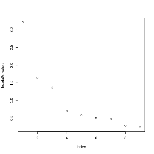 The rule of thumb is that we reject factors with an eigenvalue lower
than 1.0.
The rule of thumb is that we reject factors with an eigenvalue lower
than 1.0.
Three factors are sufficient. We now do the factor analysis again:
R
hs.efa <- fa(select(HolzingerSwineford1939, x1:x9), nfactors = 3,
             rotate = "none", fm = "ml")
hs.efa
OUTPUT
Factor Analysis using method =  ml
Call: fa(r = select(HolzingerSwineford1939, x1:x9), nfactors = 3, rotate = "none",
    fm = "ml")
Standardized loadings (pattern matrix) based upon correlation matrix
    ML1   ML2   ML3   h2   u2 com
x1 0.49  0.31  0.39 0.49 0.51 2.7
x2 0.24  0.17  0.40 0.25 0.75 2.1
x3 0.27  0.41  0.47 0.46 0.54 2.6
x4 0.83 -0.15 -0.03 0.72 0.28 1.1
x5 0.84 -0.21 -0.10 0.76 0.24 1.2
x6 0.82 -0.13  0.02 0.69 0.31 1.0
x7 0.23  0.48 -0.46 0.50 0.50 2.4
x8 0.27  0.62 -0.27 0.53 0.47 1.8
x9 0.38  0.56  0.02 0.46 0.54 1.8

                       ML1  ML2  ML3
SS loadings           2.72 1.31 0.82
Proportion Var        0.30 0.15 0.09
Cumulative Var        0.30 0.45 0.54
Proportion Explained  0.56 0.27 0.17
Cumulative Proportion 0.56 0.83 1.00

Mean item complexity =  1.8
Test of the hypothesis that 3 factors are sufficient.

df null model =  36  with the objective function =  3.05 with Chi Square =  904.1
df of  the model are 12  and the objective function was  0.08

The root mean square of the residuals (RMSR) is  0.02
The df corrected root mean square of the residuals is  0.03

The harmonic n.obs is  301 with the empirical chi square  8.03  with prob <  0.78
The total n.obs was  301  with Likelihood Chi Square =  22.38  with prob <  0.034

Tucker Lewis Index of factoring reliability =  0.964
RMSEA index =  0.053  and the 90 % confidence intervals are  0.015 0.088
BIC =  -46.11
Fit based upon off diagonal values = 1
Measures of factor score adequacy
                                                   ML1  ML2  ML3
Correlation of (regression) scores with factors   0.95 0.86 0.78
Multiple R square of scores with factors          0.90 0.73 0.60
Minimum correlation of possible factor scores     0.80 0.46 0.21
og hvilke er så med i hvilke?
R
hs.efa <- fa(select(HolzingerSwineford1939, x1:x9), nfactors = 3,
             rotate = "varimax", fm = "ml")
hs.efa
OUTPUT
Factor Analysis using method =  ml
Call: fa(r = select(HolzingerSwineford1939, x1:x9), nfactors = 3, rotate = "varimax",
    fm = "ml")
Standardized loadings (pattern matrix) based upon correlation matrix
    ML1   ML3   ML2   h2   u2 com
x1 0.28  0.62  0.15 0.49 0.51 1.5
x2 0.10  0.49 -0.03 0.25 0.75 1.1
x3 0.03  0.66  0.13 0.46 0.54 1.1
x4 0.83  0.16  0.10 0.72 0.28 1.1
x5 0.86  0.09  0.09 0.76 0.24 1.0
x6 0.80  0.21  0.09 0.69 0.31 1.2
x7 0.09 -0.07  0.70 0.50 0.50 1.1
x8 0.05  0.16  0.71 0.53 0.47 1.1
x9 0.13  0.41  0.52 0.46 0.54 2.0

                       ML1  ML3  ML2
SS loadings           2.18 1.34 1.33
Proportion Var        0.24 0.15 0.15
Cumulative Var        0.24 0.39 0.54
Proportion Explained  0.45 0.28 0.27
Cumulative Proportion 0.45 0.73 1.00

Mean item complexity =  1.2
Test of the hypothesis that 3 factors are sufficient.

df null model =  36  with the objective function =  3.05 with Chi Square =  904.1
df of  the model are 12  and the objective function was  0.08

The root mean square of the residuals (RMSR) is  0.02
The df corrected root mean square of the residuals is  0.03

The harmonic n.obs is  301 with the empirical chi square  8.03  with prob <  0.78
The total n.obs was  301  with Likelihood Chi Square =  22.38  with prob <  0.034

Tucker Lewis Index of factoring reliability =  0.964
RMSEA index =  0.053  and the 90 % confidence intervals are  0.015 0.088
BIC =  -46.11
Fit based upon off diagonal values = 1
Measures of factor score adequacy
                                                   ML1  ML3  ML2
Correlation of (regression) scores with factors   0.93 0.81 0.84
Multiple R square of scores with factors          0.87 0.66 0.70
Minimum correlation of possible factor scores     0.74 0.33 0.40
R
print(hs.efa$loadings, cutoff = 0.4)
OUTPUT
Loadings:
   ML1    ML3    ML2
x1         0.623
x2         0.489
x3         0.663
x4  0.827
x5  0.861
x6  0.801
x7                0.696
x8                0.709
x9         0.406  0.524

                 ML1   ML3   ML2
SS loadings    2.185 1.343 1.327
Proportion Var 0.243 0.149 0.147
Cumulative Var 0.243 0.392 0.539
Bum. Så har vi identificeret hvilke manifeste variable der indgår i hvilke latente faktorer.
Confirmatory factor analysis
Nu bør vi hive fat i et nyt datasæt med manifeste variable, og se hvor godt vores models latente variable beskriver variationen i det.
I praksis er de studerende (og mange andre) dovne og springer over hvor gærdet er lavest (og hvorfor pokker skulle man også vælge at springe over hvor det er højest.)
så hvordan laver man den bekræftende analyse?
Vi kal have stillet en model op. Den ser lidt speciel ud.
R
HS.model <- 'visual  =~ x1 + x2 + x3
             textual =~ x4 + x5 + x6
             speed   =~ x7 + x8 + x9'
Så fitter vi:
R
fit <- cfa(HS.model, data = HolzingerSwineford1939)
R
fit
OUTPUT
lavaan 0.6-19 ended normally after 35 iterations

  Estimator                                         ML
  Optimization method                           NLMINB
  Number of model parameters                        21

  Number of observations                           301

Model Test User Model:

  Test statistic                                85.306
  Degrees of freedom                                24
  P-value (Chi-square)                           0.000
Nej hvor er det fint. Selvfølgelig er det det. Vi har fittet vores oprindelige data på den model vi fik fra samme data. Det skal helst være ret godt.
R
summary(fit, standardized=TRUE, fit.measures=TRUE, rsquare=TRUE)
OUTPUT
lavaan 0.6-19 ended normally after 35 iterations

  Estimator                                         ML
  Optimization method                           NLMINB
  Number of model parameters                        21

  Number of observations                           301

Model Test User Model:

  Test statistic                                85.306
  Degrees of freedom                                24
  P-value (Chi-square)                           0.000

Model Test Baseline Model:

  Test statistic                               918.852
  Degrees of freedom                                36
  P-value                                        0.000

User Model versus Baseline Model:

  Comparative Fit Index (CFI)                    0.931
  Tucker-Lewis Index (TLI)                       0.896

Loglikelihood and Information Criteria:

  Loglikelihood user model (H0)              -3737.745
  Loglikelihood unrestricted model (H1)      -3695.092

  Akaike (AIC)                                7517.490
  Bayesian (BIC)                              7595.339
  Sample-size adjusted Bayesian (SABIC)       7528.739

Root Mean Square Error of Approximation:

  RMSEA                                          0.092
  90 Percent confidence interval - lower         0.071
  90 Percent confidence interval - upper         0.114
  P-value H_0: RMSEA <= 0.050                    0.001
  P-value H_0: RMSEA >= 0.080                    0.840

Standardized Root Mean Square Residual:

  SRMR                                           0.065

Parameter Estimates:

  Standard errors                             Standard
  Information                                 Expected
  Information saturated (h1) model          Structured

Latent Variables:
                   Estimate  Std.Err  z-value  P(>|z|)   Std.lv  Std.all
  visual =~
    x1                1.000                               0.900    0.772
    x2                0.554    0.100    5.554    0.000    0.498    0.424
    x3                0.729    0.109    6.685    0.000    0.656    0.581
  textual =~
    x4                1.000                               0.990    0.852
    x5                1.113    0.065   17.014    0.000    1.102    0.855
    x6                0.926    0.055   16.703    0.000    0.917    0.838
  speed =~
    x7                1.000                               0.619    0.570
    x8                1.180    0.165    7.152    0.000    0.731    0.723
    x9                1.082    0.151    7.155    0.000    0.670    0.665

Covariances:
                   Estimate  Std.Err  z-value  P(>|z|)   Std.lv  Std.all
  visual ~~
    textual           0.408    0.074    5.552    0.000    0.459    0.459
    speed             0.262    0.056    4.660    0.000    0.471    0.471
  textual ~~
    speed             0.173    0.049    3.518    0.000    0.283    0.283

Variances:
                   Estimate  Std.Err  z-value  P(>|z|)   Std.lv  Std.all
   .x1                0.549    0.114    4.833    0.000    0.549    0.404
   .x2                1.134    0.102   11.146    0.000    1.134    0.821
   .x3                0.844    0.091    9.317    0.000    0.844    0.662
   .x4                0.371    0.048    7.779    0.000    0.371    0.275
   .x5                0.446    0.058    7.642    0.000    0.446    0.269
   .x6                0.356    0.043    8.277    0.000    0.356    0.298
   .x7                0.799    0.081    9.823    0.000    0.799    0.676
   .x8                0.488    0.074    6.573    0.000    0.488    0.477
   .x9                0.566    0.071    8.003    0.000    0.566    0.558
    visual            0.809    0.145    5.564    0.000    1.000    1.000
    textual           0.979    0.112    8.737    0.000    1.000    1.000
    speed             0.384    0.086    4.451    0.000    1.000    1.000

R-Square:
                   Estimate
    x1                0.596
    x2                0.179
    x3                0.338
    x4                0.725
    x5                0.731
    x6                0.702
    x7                0.324
    x8                0.523
    x9                0.442
R
fitted(fit)
OUTPUT
$cov
      x1    x2    x3    x4    x5    x6    x7    x8    x9
x1 1.358
x2 0.448 1.382
x3 0.590 0.327 1.275
x4 0.408 0.226 0.298 1.351
x5 0.454 0.252 0.331 1.090 1.660
x6 0.378 0.209 0.276 0.907 1.010 1.196
x7 0.262 0.145 0.191 0.173 0.193 0.161 1.183
x8 0.309 0.171 0.226 0.205 0.228 0.190 0.453 1.022
x9 0.284 0.157 0.207 0.188 0.209 0.174 0.415 0.490 1.015
R
coef(fit)
OUTPUT
      visual=~x2       visual=~x3      textual=~x5      textual=~x6
           0.554            0.729            1.113            0.926
       speed=~x8        speed=~x9           x1~~x1           x2~~x2
           1.180            1.082            0.549            1.134
          x3~~x3           x4~~x4           x5~~x5           x6~~x6
           0.844            0.371            0.446            0.356
          x7~~x7           x8~~x8           x9~~x9   visual~~visual
           0.799            0.488            0.566            0.809
textual~~textual     speed~~speed  visual~~textual    visual~~speed
           0.979            0.384            0.408            0.262
  textual~~speed
           0.173
R
resid(fit, type = "normalized")
OUTPUT
$type
[1] "normalized"

$cov
       x1     x2     x3     x4     x5     x6     x7     x8     x9
x1  0.000
x2 -0.493  0.000
x3 -0.125  1.539  0.000
x4  1.159 -0.214 -1.170  0.000
x5 -0.153 -0.459 -2.606  0.070  0.000
x6  0.983  0.507 -0.436 -0.130  0.048  0.000
x7 -2.423 -3.273 -1.450  0.625 -0.617 -0.240  0.000
x8 -0.655 -0.896 -0.200 -1.162 -0.624 -0.375  1.170  0.000
x9  2.405  1.249  2.420  0.808  1.126  0.958 -0.625 -0.504  0.000
CAVE! SEMPLOT FEJLER UNDER INSTALLATION PÅ GITHUB! library(semPlot) semPaths(fit, “std”, layout = “tree”, intercepts = F, residuals = T, nDigits = 2, label.cex = 1, edge.label.cex=.95, fade = F)
Key Points
- Use
.mdfiles for episodes when you want static content - Use
.Rmdfiles for episodes when you need to generate output - Run
sandpaper::check_lesson()to identify any issues with your lesson - Run
sandpaper::build_lesson()to preview your lesson locally