Central Limit Theorem

Estimated time: 12 minutes

Overview

Questions

• How do you write a lesson using R Markdown and sandpaper?

Objectives

• Explain how to use markdown with the new lesson template

Introduction

---

An important phenomenon working with data is the “Central Limit Theorem”.

It states that, if we take a lot of samples from a distribution, the mean of those samples will approximate the normal distribution, even though the distribution in it self is not normally distributed.

The uniform distribution is not normally distributed. Without any additional arguments, it will produce x random values between 0 and 1, with equal probability for all possible values. Here we get 100 random values, and plot a histogram of them:

R

random_numbers <- runif(100) 
hist(random_numbers)

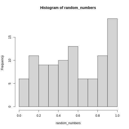This is definitely not normally distributed.

The mean of these random numbers is:

R

mean(random_numbers)

OUTPUT

[1] 0.5440314

The important point of the Central Limit Theorem is, that if we take a large number of random samples, and calculate the mean of each of these samples, the means will be normally distributed.

We could also have found the mean of the 100 random numbers like this:

R

mean(runif(100))

OUTPUT

[1] 0.521769

And we can use the replicate() function to repeat that calculation several times, in this case 1000 times:

R

repeated_means <- replicate(1000, mean(runif(100)))

When we plot the histogram of these 1000 means of 100 random numbers, we get this result:

R

hist(repeated_means)

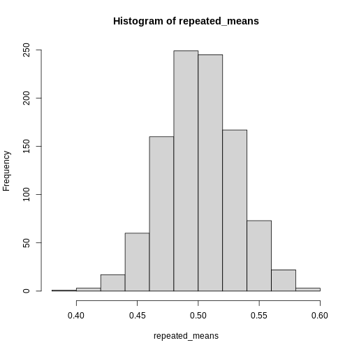
The histogram looks quite normally distributed, even though the distribution from which we drew the random samples were not.

This is the essense of the Central Limit Theorem. The distrubution of the means of our samples will approximate the normal distribution, regardless of the underlying distribution.

Because of this, we are able to treat the mean (and a number of other statistical descriptors), as normally distributed - and use the properties we know the normal distribution to have to work with them.

The math required for proving this theorem is relatively complicated, but can be found in the (extra material)[https://kubdatalab.github.io/R-toolbox/CLT-dk.html] on this page. Note that the proof is in Danish, we are working on an english version.

Key Points

• The mean of a sample can be treated as if it is normally distributed