Reproducible Data Analysis
Last updated on 2026-06-15 | Edit this page
Estimated time: 12 minutes
Overview
Questions
- How do I ensure that my results can be reproduced?
Objectives
- Explain how to use markdown
- Demonstrate how to include pieces of code
Introduction
A key concept in the scientific process is reproducibility. We should be able to run the same experiment again, and get, more or less, the same result.
We will not always get the same result, applying the same functions on the same data - some statistical techniques relies on randomness.
An example is k-means, that clusters data based on randomly selected initial centroids.
This also applies to the analysis of data. If we have a collection of measurements of blood pressure from patients before and after they have taken an antihypertensive drug, we might arrive at the result that this specific drug is not working. Doing the same analysis tomorrow, we should reach the same result.
And that can be surprisingly difficult!
There are a lot of pitfalls, ranging from accessibility to incentive structures in academia. But the three areas where R can help us are:
- Software Environment
- Documentation and Metadata
- Complex Workflows
Software Environment
Data analysis is done using specific software, libraries or packages, in a variety of versions. And it happens in an environment on the computer that might not be identical from day to day.
One example of these problems is shown every time we load tidyverse:
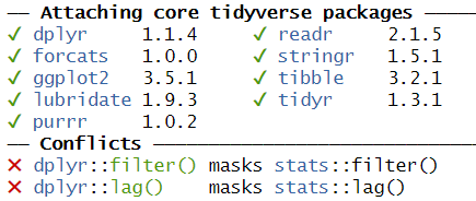
This message informs us that there is a filter()
function in the stats packages which is part of the core
R-installation. That function is masked by the filter()
function from the tidyverse´ packagedplyr`.
If our analysis relies on the way the filter() function
works in the tidyverse, we will get errors if
tidyverse is not loaded.
We might also have data stored in memory. Every time we close RStudio, we are asked if we want to save the environment:

This will save all the objects we have in our environment, in order for RStudio to be able to load them into memory when we open RStudio again.
That can be nice and useful. On the other hand we run the risk of
having the wrong version of the
my_data_that_is_ready_for_analysis dataframe lying around
in memory.
In addition we can experience performance problems. Storing a lot of large objects before closing RStudio can take a lot of time. And loading them into memory when opening RStudio will also take a lot of time.
On modern computers we normally have plenty of storage - but it is entirely possible to fill your harddrive with R-environments to the point where your computer crashes.
Documentation and Metadata
What did we actually do in the analysis? Why did we do it? Why are we reaching the conclusion we’ve arrived at?
Three very good questions. Having good metadata, data that describes your data, often makes understanding your data easier. Documenting the individual steps of your analysis, may not seem necessary right now - you know why you are doing what you are doing. But future you - you in three months, or some one else, might not remember or be able to guess (correctly).
Complex Workflows
Doing data analysis in eg Excel, can involve a lot of pointing and clicking.
And in any piece of software, the analysis will normally always involve more than one step. Those steps will have to be done in the correct order. Calculating a mean of some values, depends heavily on whether it happens before or after deleting irrelevant observations.
The solution to all of this!

Working in RMarkdown allows us to collect the text describing our data, what and why we are doing what we do, the code actually doing it, and the results of that code - all in one document.
Open a new file, choose RMarkdown, and give your document a name:

The code chunks, marked here with a light grey background, contains code, in this case not very advanced code. You can run the entire code chunk by clicking the green arrow on the right. Or by placing your cursor in the line of code you want to run, and pressing ctrl+enter (or command+enter on a Mac).
Outside the code chunks we can add our reasons for actually running
summary on the cars dataframe, and describe
what it contains.
You will see a new button in RStudio: 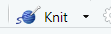
Clicking this, will “knit” your document; run each chunck of code, add the output to your document, and combine your code, the results and all your explanatory text to one html-document.
If you do not want an HTMl-document, you can knit to a MicroSoft Word document. Depending on your computer, you can knit directly to a pdf.
Having the entirety of your analysis in an RMarkdown document, and then running it, ensures that the individual steps in the analysis are run in the correct order.
It does not ensure that your documentation of what you do is written - it makes it easy to add it, but you still have to do it.
But what about the environment?
So we force ourself to have the steps in our analysis in the correct order, and we make it easy to add documentation. What about the environment?
Working with RMarkdown also adresses this problem. Every time we
knit our document, RStudio opens a new session of R,
without libraries or objects in memory. This ensures that the analysis
is done in the exact same way each and every time.
This, on the other hand, requires us to add code chunks loading libraries and data to our document.
Try it yourself
Make a new RMarkdown document, add library(tidyverse) to
the first chunk, add your own text, and change the plot to plot the
distance variable from the cars data set.
Make a new RMarkdown document - File -> New File -> R Markdown.
Change the final code chunk to include plot(cars$dist)
instead of plot(pressure), and add library(tidyverse).
- Use RMarkdown to enforce reproducible analysis