k-means
Last updated on 2026-06-15 | Edit this page
Estimated time: 12 minutes
Overview
Questions
- What is k-means?
Objectives
- Explain how to run a kmeans-clustering on data
- Demonstrate the importance of scaling
Imagine we have a set of data. We might have a lot of data on the orders from different customers in our bookshop. We would like to target our email-campaigns to them.
We do not want to go through all our customers manually. We want something automated, that partitions all our customers into eg. 10 different groups (or clusters) that are similar. Our email-campaign should focus on books about cars and WW2 when we target customers in the cluster that tend to buy that kind of books. And on other topics to other clusters.
This is a real example from a major, danish online bookseller.
This is also an example of an unsupervised clustering. We do not know the true group any given customer belongs to, and we do not want to predict which group she will end up in. We simply want to partition our data/customers into 10 groups.
In the case of the online bookseller the number was chosen to get a relatively small number of clusters, in order not to have to manage 20 or more different marketing mails. But large enough to have a decent differentation between the groups.
The number is often chose arbitrarily, but methods for choosing an “optimal” number exists.
kmeans is a way of doing this
Many unsupervised clustering algorithms exist. kmeans is just one. We provide the data, and specify the number of clusters we want to get. The algorithm will automatically provide us with them. And it will assign the datapoints to individual clusters, in a way where the datapoints have some sort of similarity of their features.
Wine as an example
We might normally use the kmeans algorithm to cluster data where we do not know the “true” clusters the data points belongs to.
In order to demonstrate the method, it is useful to have a dataset where we know the true clusters.
Here we have a dataset, where different variables, have been measured on wine made from three different types of grapes (cultivars).
The terminology differs. We have a set of columns with variables. But these variables are also often called parameters or features. Or dimensions
The dataset can be downloaded here
R
library(tidyverse)
vin <- read_csv("data/win/wine.data", col_names = F)
names(vin) <- c("cultivar",
                "Alcohol",
                "Malicacid",
                "Ash",
                "Alcalinityofash",
                "Magnesium",
                "Totalphenols",
                "Flavanoids",
                "Nonflavanoidphenols",
                "Proanthocyanins",
                "Colorintensity",
                "Hue",
                "OD280OD315ofdilutedwines",
                "Proline")
What does it do?
Before actually running the algorithm, we should probably take a look at what it does.
K-means works by chosing K - the number of clusters we want. That is a choice entirely up to us. In this example we will chose 3. Primarily because we know that there are three different cultivars.
The algorithm then choses K random points, also called centroids. In this case these centroids are in 13 dimensions, because we have 13 features in the dataset.
That makes it a bit difficult to visualize.
It then calculates the distance from each observation in the data, to each of the K centroids. After that, each observation is assigned to the centroid it is closest to. Each data point will therefore be assigned to a specific cluster, described by the relevant centroid.
The algorithm then calculates three new centroids. All the observations assigned to centroid A are averaged, and we get a new centroid. The same calculations are done for the other two centroids, and we now have three new centroids. They now actually have a relation to the data - before they were assigned randomly, now they are based on the data.
Now the algorithm repeats the calculation of distance. For each observation in the data, which of the new centroids is it closest to it. Since we calculated new centroids, some of the observations will switch and will be assigned to a new centroid.
Again the new assignments of observations are used to calculate new centroids for the three clusters, and all these calculations are repeated until no observations swithces between clusters, or we have repeated the algorithm a set number of times (by default 10 times).
After that, we have clustered our data in three (or whatever K we chose) clusters, based on the features of the data.
How do we actually do that?
The algorithm only works with numerical data.
Let us begin by removing the variable containing the true answers.
R
cluster_data <- vin |>
  select(-cultivar)
There are only numerical values in this example, so we do not have to remove other variables.
After that, we can run the function kmeans, and specify
that we want three centers (K), and save the result to an object, that
we can work with afterwards:
R
clustering <- kmeans(cluster_data, centers = 3)
clustering
OUTPUT
K-means clustering with 3 clusters of sizes 69, 62, 47

Cluster means:
   Alcohol Malicacid      Ash Alcalinityofash Magnesium Totalphenols Flavanoids
1 12.51667  2.494203 2.288551        20.82319  92.34783     2.070725   1.758406
2 12.92984  2.504032 2.408065        19.89032 103.59677     2.111129   1.584032
3 13.80447  1.883404 2.426170        17.02340 105.51064     2.867234   3.014255
  Nonflavanoidphenols Proanthocyanins Colorintensity       Hue
1           0.3901449        1.451884       4.086957 0.9411594
2           0.3883871        1.503387       5.650323 0.8839677
3           0.2853191        1.910426       5.702553 1.0782979
  OD280OD315ofdilutedwines   Proline
1                 2.490725  458.2319
2                 2.365484  728.3387
3                 3.114043 1195.1489

Clustering vector:
  [1] 3 3 3 3 2 3 3 3 3 3 3 3 3 3 3 3 3 3 3 2 2 2 3 3 2 2 3 3 2 3 3 3 3 3 3 2 2
 [38] 3 3 2 2 3 3 2 2 3 3 3 3 3 3 3 3 3 3 3 3 3 3 1 2 1 2 1 1 2 1 1 2 2 2 1 1 3
 [75] 2 1 1 1 2 1 1 2 2 1 1 1 1 1 2 2 1 1 1 1 1 2 2 1 2 1 2 1 1 1 2 1 1 1 1 2 1
[112] 1 2 1 1 1 1 1 1 1 2 1 1 1 1 1 1 1 1 1 2 1 1 2 2 2 2 1 1 1 2 2 1 1 2 2 1 2
[149] 2 1 1 1 1 2 2 2 1 2 2 2 1 2 1 2 2 1 2 2 2 2 1 1 2 2 2 2 2 1

Within cluster sum of squares by cluster:
[1]  443166.7  566572.5 1360950.5
 (between_SS / total_SS =  86.5 %)

Available components:

[1] "cluster"      "centers"      "totss"        "withinss"     "tot.withinss"
[6] "betweenss"    "size"         "iter"         "ifault"
This is a bit overwhelming. The centroids in the three clusters are defined by their mean values of all the dimensions/variables in them. We can see that there appears to be a difference between the alcohol content between all of the three clusters. Whereas the difference between cluster 1 and 3 for malicacid is very close.
We also get at clustering vector, that gives the number of the cluster each datapoint is assigned to. And we get some values for the variation between the clusters.
How well did it do?
We know the true values, so we extract the clusters the algorithm found, and match them with the true values:
R
testing_clusters <- tibble(quess = clustering$cluster,
                           true = vin$cultivar)
And count the matches:
R
table(testing_clusters)
OUTPUT
     true
quess  1  2  3
    1  0 50 19
    2 13 20 29
    3 46  1  0
The algorithm have no idea about how the true groups are numbered, so the numbering does not match. But it appears that i does a relatively good job on two of the types of grapes. and is a bit confused about the third.
Does that mean the algorithm does a bad job?
Preprocessing is necessary!
Looking at the data give a hint about the problems:
R
head(vin)
OUTPUT
# A tibble: 6 × 14
  cultivar Alcohol Malicacid   Ash Alcalinityofash Magnesium Totalphenols
     <dbl>   <dbl>     <dbl> <dbl>           <dbl>     <dbl>        <dbl>
1        1    14.2      1.71  2.43            15.6       127         2.8
2        1    13.2      1.78  2.14            11.2       100         2.65
3        1    13.2      2.36  2.67            18.6       101         2.8
4        1    14.4      1.95  2.5             16.8       113         3.85
5        1    13.2      2.59  2.87            21         118         2.8
6        1    14.2      1.76  2.45            15.2       112         3.27
# ℹ 7 more variables: Flavanoids <dbl>, Nonflavanoidphenols <dbl>,
#   Proanthocyanins <dbl>, Colorintensity <dbl>, Hue <dbl>,
#   OD280OD315ofdilutedwines <dbl>, Proline <dbl>
Note the differences between the values of “Malicacid” and “Magnesium”. One have values between 0.74 and 5.8 and the other bewtten 70 and 162. The latter influences the means much more that the former.
It is therefore good practice to scale the features to have the same
range and standard deviation. A function scale() that does
exactly that exists in R:
R
scaled_data <- scale(cluster_data)
If we now do the same clustering as before, but now on the scaled data, we get much better results:
R
set.seed(42)
clustering <- kmeans(scaled_data, centers = 3)
tibble(quess = clustering$cluster, true = vin$cultivar) |>
  table()
OUTPUT
     true
quess  1  2  3
    1 59  3  0
    2  0 65  0
    3  0  3 48
By chance, the numbering of the clusters now matches the “true” cluster numbers.
The clustering is not perfect. 3 observations belonging to cluster 2, are assigned to cluster 1 by the algorithm (and 3 more to cluster 3).
In this caase we know the true values. Had we not, we would still have gotten the same groups, and could have correctly grouped the different data points.
What are those distances?
It is easy to measure the distance between two observations when we only have two features/dimensions: Plot them on a piece of paper, and bring out the ruler.
But what is the distance between this point:
1, 14.23, 1.71, 2.43, 15.6, 127, 2.8, 3.06, 0.28, 2.29, 5.64, 1.04, 3.92, 1065
and this one:
1, 13.2, 1.78, 2.14, 11.2, 100, 2.65, 2.76, 0.26, 1.28, 4.38, 1.05, 3.4, 1050?
Rather than plotting and measuring, if we only have two observations with two features, and we call the the observations \((x_1, y_1)\) and \((x_2,y_2)\) we can get the distance using this formula:
\[d = \sqrt{(x_2 - x_1)^2 + (y_2 - y_1)^2} \]
For an arbitrary number of dimensions we get this: \[d = \sqrt{\sum_{i=1}^{n} \left(x_2^{(i)} - x_1^{(i)}\right)^2}\]
Where the weird symbol under the squareroot sign indicates that we add all the squared differences between the pairs of observations.
Is the clustering reproducible?
Not nessecarily. If there are very clear clusters, in general it will be.
But the algorithm is able to find clusters even if there are none:
Here we have 1000 observations of two features:
R
test_data <- data.frame(x = rnorm(1000), y = rnorm(1000))
They are as random as the random number generator can do it.
Let us make one clustering, and then another:
R
set.seed(47)
kmeans_model1 <- kmeans(test_data, 5)
kmeans_model2 <- kmeans(test_data, 5)
And then extract the clustering and match them like before:
R
tibble(take_one = kmeans_model1$cluster,
        take_two = kmeans_model2$cluster) |>
table()
OUTPUT
        take_two
take_one   1   2   3   4   5
       1   2 132   0  23   0
       2   2   0 217   0   2
       3   0   0  11   1 124
       4 127  73   9   0   0
       5   0  68   1 121  87
Two clusterings on the exact same data. And they are pretty different.
Do not be confused by the fact that take_one-group-4 matches rather well with take_two-group-1. The numbering is arbitrary.
Visualizing it makes it even more apparent:
R
tibble(take_one = kmeans_model1$cluster,
        take_two = kmeans_model2$cluster)  |>
  cbind(test_data) |>
ggplot(aes(x,y,colour= factor(take_one))) +
geom_point()
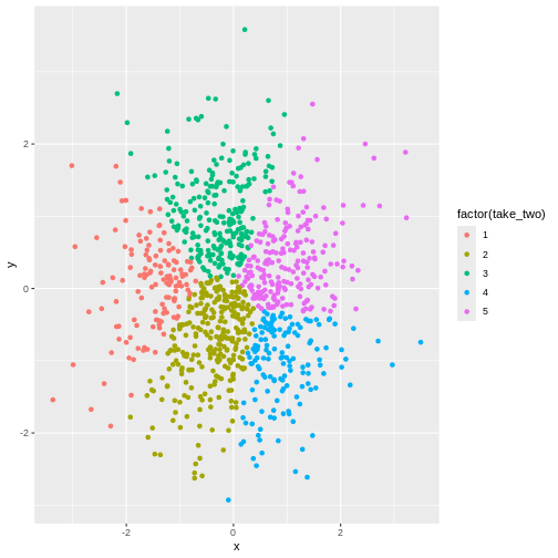
R
tibble(take_one = kmeans_model1$cluster,
        take_two = kmeans_model2$cluster)  |>
  cbind(test_data) |>
ggplot(aes(x,y,colour= factor(take_two))) +
geom_point()

In other words - the algorithm will find clusters. And the clustering depends, to a certain degree on the random choice of initial centroids.
Can it be use on any data?
No. Even though there might actually be clusters in the data, the
algorithm is not necessarily able to find them. Consider this data:
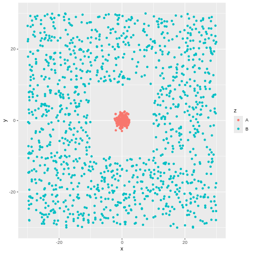 There is obviously a cluster centered around (0,0). And another cluster
more or lesss evenly spread around it.
There is obviously a cluster centered around (0,0). And another cluster
more or lesss evenly spread around it.
The algorithm will find two clusters:
R
library(tidymodels)
kmeans_model3 <- kmeans(test_data[,-3], 2)
cluster3 <- augment(kmeans_model3, test_data[,-3])
ggplot(cluster3, aes(x,y,colour=.cluster)) +
  geom_point()
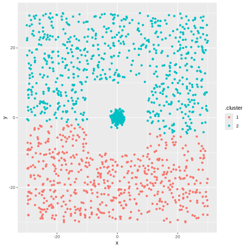 But not the ones we want.
- kmeans is an unsupervised technique, that will find the hidden structure in our data that we do not know about
- kmeans will find the number of clusters we ask for. Even if there is no structure in the data at all