How is the data distributed?
Last updated on 2026-06-15 | Edit this page
Estimated time: 12 minutes
Overview
Questions
- If my data is not normally distributed - which distribution does it actually follow?
Objectives
- Show how to identify possible distributions describing the data
Introduction
Your data was not normally distributed. Now what?
The process generating your data is probably following some distribution. The size distribution of cities appears to follow a Pareto distibution, as is wealth. The number of mutations in a string of DNA appears to follow a poisson distribution. And the distribution of wind speeds as well as times to failure for technical components both follow the Weibull distribution.
If you have a theoretical foundation for which distribution you data generating function follows, that is nice.
If you do not - we will be interested in figuring out which distribution your data actually follow.
How?
We fit our data to a distribution. Or rather - we fit the data to several different distributions and then choose the best.
Let us look at some data. The faithful data set contains
272 observations of the Old Faithful geyser in Yellowstone National Park
in USA. We only look at eruptions that lasts longer than 3 minutes:
R
library(tidyverse)
eruption_example <- faithful |>
  filter(eruptions > 3) |>
  dplyr::select(eruptions)
Det er nødvendigt at specificere at vi bruger
dplyr::select da den maskeres af MASS-pakken
Rather than testing a lot of different distributions, we can use the
gamlss package, and two add-ons to that.
R
library(gamlss)
library(gamlss.dist)
library(gamlss.add)
gamlss has the advantage of implementing a lot
of different statistical distributions.
The function fitDist() from gamlss will fit
the data to a selection of different statistical distributions,
calculate a measure of the goodness of fit, and return the best fit (and
information on all the others). Rather than testing against all 97
different distributions supported by gamlss, we can specify
only a selection, in this case realplus, that only includes
the 23 distributions that are defined for positive, real numbers:
R
fit <- fitDist(eruptions, type = "realplus", data = eruption_example)
OUTPUT
| | | 0% | |=== | 4% | |====== | 9% | |========= | 13% | |============ | 17%OUTPUT
| |=============== | 22% | |================== | 26% | |===================== | 30% | |======================== | 35% | |=========================== | 39% | |============================== | 43%OUTPUT
| |================================= | 48%OUTPUT
| |===================================== | 52%OUTPUT
| |======================================== | 57% | |=========================================== | 61% | |============================================== | 65% | |================================================= | 70% | |==================================================== | 74%OUTPUT
  |                                                                              |=======================================================               |  78%  |                                                                              |==========================================================            |  83%Error in solve.default(oout$hessian) :
  Lapack routine dgesv: system is exactly singular: U[4,4] = 0
  |                                                                              |=============================================================         |  87%Error in solve.default(oout$hessian) :
  Lapack routine dgesv: system is exactly singular: U[4,4] = 0
  |                                                                              |================================================================      |  91%  |                                                                              |===================================================================   |  96%  |                                                                              |======================================================================| 100%
If you do this yourself, you will notice a lot of error-messages. It is not possible to fit this particular data to all the distributions, and the ones where the fit fails (enough), we will get an error message.
The output from fitDist() will return the best fit:
R
fit
OUTPUT
Family:  c("WEI2", "Weibull type 2")
Fitting method: "nlminb"

Call:  gamlssML(formula = y, family = DIST[i])

Mu Coefficients:
[1]  -18.69
Sigma Coefficients:
[1]  2.524

 Degrees of Freedom for the fit: 2 Residual Deg. of Freedom   173
Global Deviance:     175.245
            AIC:     179.245
            SBC:     185.574
We are told that the statistical distribution that best fits the data
is Weibull type 2 and that the AIC-measurement of goodness
of fit is 170.245.
Is that a good fit? That is a good question. It strongly depends on the values in the dataset. In this dataset, the length of the eruptions are measured in minutes If we choose to measure that length in another unit, eg seconds, the distribution should not change. But the AIC will.
We can use the AIC to decide that one distribution fits the data better than another, but not to conclude that that distribution is the correct one.
The fit object containing the output of the
fitDist() function contains quite a bit more.
If we start by getting the errors out of the way,
fit$failed returns the two distributions that failed enough
to cause errors:
R
fit$failed
OUTPUT
[[1]]
[1] "GIG"

[[2]]
[1] "LNO"
As mentioned fitDist() fitted the data to 23 different
distributions. We can inspect the rest, and their associated AIC-values
like this:
R
fit$fits
OUTPUT
    WEI2     WEI3      WEI       GG    BCPEo     BCPE    BCCGo     BCCG
179.2449 179.2449 179.2449 181.1349 181.4953 181.4953 183.1245 183.1245
     GB2     BCTo      BCT   exGAUS       GA   LOGNO2    LOGNO       IG
183.1358 185.1245 185.1245 190.2994 194.4665 198.3047 198.3047 198.3558
  IGAMMA      EXP  PARETO2       GP PARETO2o
202.6759 861.8066 863.8067 863.8067 863.8071
Here we get WEI2 first, with an AIC of 179.2449, but we
can see that WEI3 and WEI1 have almost exactly
the same AIC. Not that surprising if we guess that
Weibull type 3 is probably rather similar to
Weibull type 2.
The difference in AIC for the first two distributions tested is very
small. Is it large enough for us to think that WEI2 is
significantly better than WEI3?
No. As a general rule of thumb, the difference between the AIC of two distributions have to be larger than 2 for us to see a significant difference.
We can get more details using the summary()
function:
R
summary(fit)
OUTPUT
*******************************************************************
Family:  c("WEI2", "Weibull type 2")

Call:  gamlssML(formula = y, family = DIST[i])

Fitting method: "nlminb"


Coefficient(s):
             Estimate  Std. Error  t value   Pr(>|t|)
eta.mu    -18.6934274   1.1306427 -16.5334 < 2.22e-16 ***
eta.sigma   2.5242093   0.0589965  42.7858 < 2.22e-16 ***
---
Signif. codes:  0 '***' 0.001 '**' 0.01 '*' 0.05 '.' 0.1 ' ' 1

 Degrees of Freedom for the fit: 2 Residual Deg. of Freedom   173
Global Deviance:     175.245
            AIC:     179.245
            SBC:     185.574
And we can get at graphical description as well:
R
plot(fit)
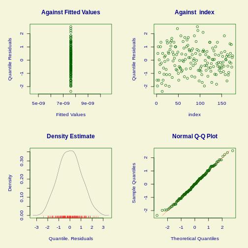
OUTPUT
******************************************************************
	      Summary of the Quantile Residuals
                           mean   =  -0.001205749
                       variance   =  0.9953007
               coef. of skewness  =  0.09022876
               coef. of kurtosis  =  2.529951
Filliben correlation coefficient  =  0.9976953
******************************************************************
What about the other options?
General comments
Above we got the “best” fit. But we also noted that in order for us to conclude that one distribution is a better fit than another, the difference in AIC should be at least 2.
What we are looking for might not actually be the probability distribution that best fits our data. Our data might be noisy or there might me systematic errors. The probability distribution we really want, is the one that best matches the underlying data generating function, the mechanisms in the real world that we are studying, that actually is at the hearth of the data we collect.
We might not be able to find that. But we should consider if some of
the other possibilities provided by fitDist() might
actually be better.
Og her er det vi holder dem fast på at det faktisk er dem selv der er de bedst kvalificerede til at afgøre det. For det er dem der forstår domænet og data.
First step is to look at the relevant distributions. In the setup
with gamlss, gamlss.dist and
gamlss.add we can test distributions of different types.
The complete list can be found using the help function for
fitDist(), but falls in the following families:
- realline - continuous distributions for all real values
- realplus - continuous distributions for positive real values
- realAll - all continuous distributions - the combination of realline and realplus
- real0to1 - continuous distributions defined for real values between 0 and 1
- counts - distributions for counts
- binom - binomial distributions
Begin by considering which type whatever your data is describing, best matches.
Actually looking at the fits
For the selection of eruptions that we fitted, we chose the “realplus” selection of distibutions to test. We did that, because the eruption times are all positive, and on the real number line.
“Real numbers”, på dansk reelle tal. Hvis du ved hvad imaginære tal er, ved du også hvad reelle tal er. Hvis ikke - så er reelle tal alle de tal du vil tænke på som tal.
Behind the scenes fitDist fits the data to the chosen
selection of distributions, and returns the best.
Looking at the result of the fit we see this:
R
fit
OUTPUT
Family:  c("WEI2", "Weibull type 2")
Fitting method: "nlminb"

Call:  gamlssML(formula = y, family = DIST[i])

Mu Coefficients:
[1]  -18.69
Sigma Coefficients:
[1]  2.524

 Degrees of Freedom for the fit: 2 Residual Deg. of Freedom   173
Global Deviance:     175.245
            AIC:     179.245
            SBC:     185.574
In the Call part of the output, we see this:
Call: gamlssML(formula = y, family = DIST[i])
and from that we can deduces that if we want to fit the data to eg the log-normal distribution (in the documentation we find that the abbreviation for that is “LOGNO”), we can do it like this:
R
log_norm_fit <- gamlss(eruptions ~ 1, family = LOGNO, data = eruption_example)
OUTPUT
GAMLSS-RS iteration 1: Global Deviance = 194.3047
GAMLSS-RS iteration 2: Global Deviance = 194.3047
R
summary(log_norm_fit)
OUTPUT
******************************************************************
Family:  c("LOGNO", "Log Normal")

Call:
gamlss(formula = eruptions ~ 1, family = LOGNO, data = eruption_example)

Fitting method: RS()

------------------------------------------------------------------
Mu link function:  identity
Mu Coefficients:
            Estimate Std. Error t value Pr(>|t|)
(Intercept) 1.451832   0.007461   194.6   <2e-16 ***
---
Signif. codes:  0 '***' 0.001 '**' 0.01 '*' 0.05 '.' 0.1 ' ' 1

------------------------------------------------------------------
Sigma link function:  log
Sigma Coefficients:
            Estimate Std. Error t value Pr(>|t|)
(Intercept) -2.31561    0.05345  -43.32   <2e-16 ***
---
Signif. codes:  0 '***' 0.001 '**' 0.01 '*' 0.05 '.' 0.1 ' ' 1

------------------------------------------------------------------
No. of observations in the fit:  175
Degrees of Freedom for the fit:  2
      Residual Deg. of Freedom:  173
                      at cycle:  2

Global Deviance:     194.3047
            AIC:     198.3047
            SBC:     204.6343
******************************************************************- The data generating function is not necessarily the same as the distribution that best fit the data
- Chose the distribution that best describes your data - not the one that fits best