Linear regression
Last updated on 2026-06-15 | Edit this page
Estimated time: 12 minutes
Overview
Questions
- How do I make a linear regression?
- How do I interpret the results of a linear regression?
Objectives
- Explain how to fit data to a linear equation in one dimension
Introduction
Here is some data, observations of the distance (in ft) it takes to stop a car driving at different speeds (in mph):
R
library(tidyverse)
OUTPUT
── Attaching core tidyverse packages ──────────────────────── tidyverse 2.0.0 ──
✔ dplyr     1.2.1     ✔ readr     2.2.0
✔ forcats   1.0.1     ✔ stringr   1.6.0
✔ ggplot2   4.0.3     ✔ tibble    3.3.1
✔ lubridate 1.9.5     ✔ tidyr     1.3.2
✔ purrr     1.2.2
── Conflicts ────────────────────────────────────────── tidyverse_conflicts() ──
✖ dplyr::filter() masks stats::filter()
✖ dplyr::lag()    masks stats::lag()
ℹ Use the conflicted package (<http://conflicted.r-lib.org/>) to force all conflicts to become errors
R
cars |>
  ggplot(aes(speed,dist)) +
  geom_point()
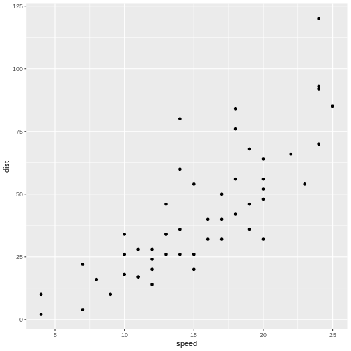
Not surprisingly the faster the car travels, the longer distance it takes to stop it.
If we want to predict how long a car traveling at 10 mph takes to stop, we could look at the observations at 10 mph and note that there is some variation. We might take the average of those observations, and use that as an estimate of how many feet it takes to stop a car traveling at 10 mph.
But what if we want to predict how long it takes to stop the car if we are driving it at 12.5 mph instead? That would be nice to know, in order to avoid hitting stuff. There are no observations in the data at 12.5 mph! We could estimate it as the average of the (average) stopping distance at 12 mph and at 13 mph (21.5 and 35 ft respectively) and give an estimate of 28.25 ft.
This is easy - 12.5 is exactly at the middle of the interval of 12 to 13 mph. But what if we want the distance at 12.4 mph?
Instead of fiddling with the numbers manually, we note that it appears to be possible to draw a straight line through the points, describing the connection between the two variables.
Let’s do that:
R
cars |>
  ggplot(aes(speed,dist)) +
  geom_point() +
  geom_smooth(method = "lm", se = F)
OUTPUT
`geom_smooth()` using formula = 'y ~ x'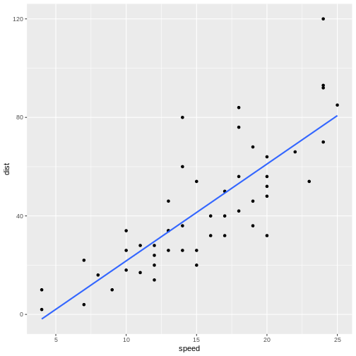
The points do not fall precisely on the line, but it’s not very bad.
Bremselængden er faktisk ikke en lineær funktion af hastigheden. Bilen har kinetisk (bevægelses) energi så længe den bevæger sig. Den skal vi have ned på 0. Og eftersom den kinetiske energi er givet ved \(E_{kin} = \frac{1}{2}mv^2\) hvor m er bilens masse og v er hastigheden, vil dist afhænge af speed i anden.
When we want to figure out how long it takes to stop a car driving at 12.5 mph, we can locate 12.5 on the x-axis, move vertically up to the line, and read the corresponding value on the y-axis, about 30 mph.
But we can do better. Such a line can be described mathematically. Straight lines in two dimensions can in general be described using the formula:
\[ y = ax + b \] or, in this specific case:
\[ dist = a*speed + b \]
a and b are the coefficients of this
“model”. a is the slope, or how much the distance changes,
if we change speed by one. b is the intercept, the value
where the line crosses the y-axis. Or the distance it takes to stop a
car, traveling at a speed of 0 miles per hour - a value that does not
necessarily make sense, but is still a part of the model.
If we want to be very strict about it, that = is not
really equal. The expression describes the straight line, but the actual
observations do not actually fall on the line. If, for a given dist and
speed, we want the expression to actually be equal, there is some
variation that we need to include. We do that by adding a
residual:
\[ dist = a*speed + b + \epsilon \]
And, if we want to be very mathematical concise, instead of using
aand b for the coefficients in the expression,
we would instead write it like this:
\[ dist = \beta_0 + \beta_1 speed + \epsilon \]
That is all very nice. But how do we find the actual a
and b (or \(\beta_i\))?
What is the “best” line or model for this?
We do that by fitting a and b to values
that minimizes \(\epsilon\), that is,
we need to find the difference between the actual observed values, and
the prediction from the expression or model. Instead of looking at the
individual differences one by one, we look at the sum of the
differences, and minimizes that. However, the observed values can be
larger than the prediction, or smaller. The differences can therefore be
both negative and positive, and the sum can become zero because the
difference might cancel each other out.
To avoid that problem, we square the differences, and then minimize
the sum of the squares. That is the reason for calling the method for
minimizing \(\epsilon\), and by that
finding the optimal a and b, “least
squares”.
In a simple linear model like this, we can calculate the coefficients directly:
\[\beta_1 = \frac{\sum_{i=1}^{n} (x_i - \overline{x})(y_i - \overline{y})}{\sum_{i=1}^{n} (x_i - \overline{x})^2}\]
\[\beta_0 = \overline{y} - \beta_1\overline{x}\]
We do not want to do that - R can do it for us, with the function
lm()
R
lm(y~x, data = data)
y~x is the “formula notation” in R, and describes that y is a function of x.
Using the example from above:
R
linear_model <- lm(dist~speed, data = cars)
We saved the result of the function in an object, in order to be able to work with it. If we just want the coefficients, we can output the result directly:
R
linear_model
OUTPUT
Call:
lm(formula = dist ~ speed, data = cars)

Coefficients:
(Intercept)        speed
    -17.579        3.932
This gives us the coefficients of the model. The intercept,
b or \(\beta_0\) is
-17.579. And the slope, a or \(\beta_1\) is 3.932.
Having a negative intercept, or in this case any intercept different from 0 does not make physical sense - a car travelling at 0 miles pr hour should have a stopping distance of 0 ft.
The slope tells us, that if we increase the speed of the car by 1 mph, the stopping distance will increase by 3.932 ft.
Challenge 1: Can you do it?
What stopping distance does the model predict if the speed i 12.5 mph?
3.932*12.5 - 17.579 = 31.571 ft
Challenge 2: Might there be a problem with that prediction?
Yep. We might be able to measure the speed with the implied precision. But the prediction implies a precision on the scale of 1/10000 mm.
We can get more details using the summary()
function:
R
summary(linear_model)
OUTPUT
Call:
lm(formula = dist ~ speed, data = cars)

Residuals:
    Min      1Q  Median      3Q     Max
-29.069  -9.525  -2.272   9.215  43.201

Coefficients:
            Estimate Std. Error t value Pr(>|t|)
(Intercept) -17.5791     6.7584  -2.601   0.0123 *
speed         3.9324     0.4155   9.464 1.49e-12 ***
---
Signif. codes:  0 '***' 0.001 '**' 0.01 '*' 0.05 '.' 0.1 ' ' 1

Residual standard error: 15.38 on 48 degrees of freedom
Multiple R-squared:  0.6511,	Adjusted R-squared:  0.6438
F-statistic: 89.57 on 1 and 48 DF,  p-value: 1.49e-12
Let us look at that output in detail.
Call simply repeats the model that we build, just in
case we have forgotten it - but also to have the actual model included
in the output, in order for other functions to access it and use it. We
will get to that.
The residuals are included. It is often important to take a look at those, and we will do that shortly.
Now, the coefficients.
The estimates for intercept and speed, that is the intercept and the slope of the line, are given. Those are the same we saw previously. We also get a standard error. We need that for testing how much trust we have in the result.
We are almost certain that the estimates of the values for intercept and slope are not correct. They are estimates after all and we will never know what the true values are. But we can test if they are zero.
The hypothesis we can test is - is the coefficient for the slope actually zero, even though the estimate we get is 3.9? If it is zero, speed will not have any influence on the stopping distance. So; with what certainty can we rule out that it is in fact zero?
We are testing the hypothesis that we have gotten a value for speed of 3.9 by random chance, but that the true value is zero. If it is zero, the value of 3.9 is 9.5 standard errors away from 0: 3.9324/0.4155 = 9.46426. And, using the t-distribution which describes these sorts of things pretty well, that will happen very rarely. The Pr, or p-value, is 1.49e-12. That is the chance, or probability, that we will get a value for the slope in our model that is 9.464 standard errors away from zero, if the true value of the slope is zero.
In general if the p-value is smaller than 0.05, we reject the hypothesis that the true value of the slope is 0.
Since we can assume that the estimates are normally distributed, we can see that, if the true value of the slope was zero, the value we get here, is 3.9324/0.4155 = 9.46426, standard errors away from zero.
RSE is the squareroot of the sum of the squared residuals, divided by the number of observations, \(n\) minus the number of parameters in the model, in this case 2. It is an estimate of the average difference between the observed values, and the values the model predicts. We want RSE to be as small as possible. What is small? That depends on the size of the values. If we predict values in the range of 0 to 2, an RSE of 15 is very large. If we predict values in the range 0 to 1000, it is small.
Multiple R-squared, is a measure of how much of the variation in
dist that our model explains. In this case the model
explains ~65% of the variation. Not that impressive, but acceptable.
The adjusted R-squared adjusts the multiple R-square by the number of independent variables in the model. It becomes an important measure of how good the model is, when we get to multiple linear regression, because we will get a better R-squared by adding independent variables, even if these variables do not actually have any connection to the dependent variables.
The F-statistic is 89.57 and has a p-value of 1.49e-12.
This tests our model against a model where all the slopes (we only have one in this case) are 0; that is, is the overall model significant. In this case it is, and there is overall strong evidence for the claim that the speed of the car influences the stopping distance.
Challenge
Make a model, where you describe the length of the flipper of a
penguin, as a function of its weigth. You find data on penguins in the
library palmerpenguins.
R
library(palmerpenguins)
OUTPUT
Attaching package: 'palmerpenguins'OUTPUT
The following objects are masked from 'package:datasets':

    penguins, penguins_raw
R
penguin_model <- lm(flipper_length_mm~body_mass_g, data = penguins)
summary(penguin_model)
OUTPUT
Call:
lm(formula = flipper_length_mm ~ body_mass_g, data = penguins)

Residuals:
     Min       1Q   Median       3Q      Max
-23.7626  -4.9138   0.9891   5.1166  16.6392

Coefficients:
             Estimate Std. Error t value Pr(>|t|)
(Intercept) 1.367e+02  1.997e+00   68.47   <2e-16 ***
body_mass_g 1.528e-02  4.668e-04   32.72   <2e-16 ***
---
Signif. codes:  0 '***' 0.001 '**' 0.01 '*' 0.05 '.' 0.1 ' ' 1

Residual standard error: 6.913 on 340 degrees of freedom
  (2 observations deleted due to missingness)
Multiple R-squared:  0.759,	Adjusted R-squared:  0.7583
F-statistic:  1071 on 1 and 340 DF,  p-value: < 2.2e-16
Testing the assumptions
We can always make a linear model. The questions is: should we?
There are certain assumptions that needs to be met in order to trust a linear model.
There should be a linear connection between the dependent and independent variable. We test that by comparing the observed values with the predicted values (the straight line).
Independence. The observations needs to be independent. If one measurement influences another measurement, we are not allowed to use a linear model.
Normality of residuals. The residuals must be normally distributed.
The three assumptions can be formulated in different ways, and it can be useful to read more than one in order to understand them. This is a different way:
- For any given value of x, the corresponding value of y has an average value of \(\alpha + \beta x\)
- For any two data points, the error terms are independent of each other.
- For any given value of x, the corresponding value of y is normally distributed about \(\alpha + \beta x\) with the same variance \(\sigma^2\) for any x
In general we know our data well enough to determine if the first two
are fulfilled. The third assumptions can be tested using a
qqplot. We begin by extracting the residuals from our
model:
R
residuals <- residuals(linear_model)
And then plotting them:
R
qqnorm(residuals)
qqline(residuals)
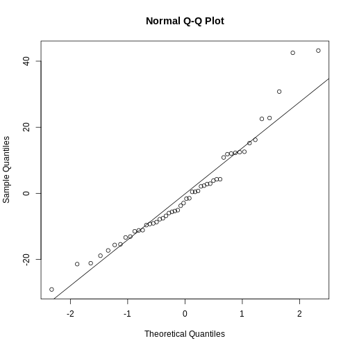
The points should be (close to be) on the straight line in the plot. In this case they are close enough.
This is also a handy way to test if our data is normally distributed.
Challenge
Test if the residuals in our penguin model from before, are normally distributed.
R
penguin_residuals <- residuals(penguin_model)
qqnorm(penguin_residuals)
qqline(penguin_residuals)
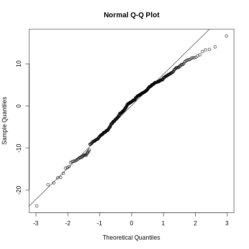 They are relatively close to normal.
- Linear regression show the (linear) relationship between variables.
- The assumption of normalcy is on the residuals, not the data!